library(modelsummary) # for tables
options(modelsummary_model_labels_term = "Parameter") # for increased accessibility
library(kableExtra) # for tables
This book is in Open Review. I want your feedback to make the book better for you and other readers. To add your annotation, select some text and then click the on the pop-up menu. To see the annotations of others, click the in the upper right hand corner of the page
7 Causal Inference
In this section, I will provide a very brief introduction to some of the concepts and tools used to evaluate evidence for causal effects from observational data.
Learning objectives
- Gain a deeper appreciation for why correlation (or association) is not the same as causation
- Discover basic rules that allow one to determine dependencies (correlations) among variables from an assumed causal network
- Understand how causal networks can be used to inform the choice of variables to include in a regression model
Credit: this section was heavily influenced by Daniel Kaplan’s chapter on Causation in his Statistics: A Fresh Approach (Kaplan 2009) and the excellent introduction to causal inference (Dablander 2020) from which many of the examples are drawn.
7.1 R Packages
We begin by loading a few packages upfront:
In addition, we will explore functions for evaluating conditional (in)dependencies in a Directed Acyclial Graph (DAG) using the ggm package (Marchetti et al. 2020).
7.2 Introduction to causal inference
Most of the methods covered in introductory and even advanced statistics courses focus on methods for quantifying associations. For example, the regression models covered in this course quantify linear and non-linear associations between explanatory (\(X_1, X_2, \ldots, X_k\)) variables and a response variable (\(Y\)). Yet, most interesting research questions emphasize understanding the causes underlying the patterns we observe in nature, and information about causes and effects are critical for informing our thinking, decision making, government policies, etc. For example, an understanding of causation is needed to answer questions about:
What will happen if we intervene in a system or manipulate one or more variables in some way (e.g., will we increase our longevity if we take a daily vitamin? Will we cause more businesses to leave the state if we increase taxes? How will a vaccine mandate influence disease transmission, unemployment rates, etc? Will we be able to reduce deer herds if we require hunters to shoot a female deer before they can harvest a male deer (sometimes referred to as an earn-a-buck management strategy1)?
Scenarios that we will never be able to observe (e.g., would George Floyd still be alive today had he been white? Would your female friend or neighbor have been promoted if she had been male? Would there have been fewer bird collisions with the Vikings stadium if it had been built differently?); These types of questions involve counterfactuals - and require considering what might have happened in an alternative world where the underlying conditions were different (e.g., where George Floyd was white, your neighbor was a male, or if the Viking stadium had been built differently).
Importantly, we can’t answer these questions using information on associations alone. For example, if we observe that \(X\) and \(Y\) are correlated, this could be due to \(X\) causing \(Y\), \(Y\) causing \(X\), or some other variable (or set of variables) causing both \(X\) and \(Y\). Answers to questions like those above also may require consideration of both direct and indirect effects. For example, consider whether increasing taxes on businesses will increase the likelihood that they will locate to another state. Increasing taxes will almost surely have a direct negative effect on the likelihood of keeping a business in the state since no CEO wants to voluntarily pay more taxes to the government. On the other hand, taxes may have a positive indirect effect if the government spends its money wisely. For example, strong public schools, updated roads and bridges, and access to parks and trails may all help businesses attract skilled workers.
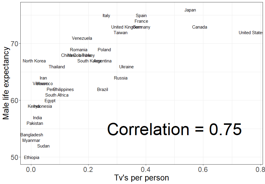
When you took a introductory statistics class, you probably heard your instructor say at least once, “correlation is not causation.” Furthermore, you probably learned about some of the challenges associated with inferring causation from observational data and the benefits of performing experiments whenever possible to establish causal linkages. A key challenge with inferring causation from observational data is that there are almost always confounding variables (variables correlated with both the predictor of interest and the response variable) that could offer an alternative explanation for why the predictor and response variables are correlated. One of my favorite examples of confounding is from Lock et al. (2020) (Figure 7.1), simply because it lets me talk about my father-in-law and the fact that he has collected a large number of old televisions. If you look at the average life expectancy versus the number of televisions (TVs) per person in different countries, there is a clear positive correlation (Figure 7.1). Does that mean my father-in-law will live forever thanks to his stockpiles of TVs? Should we all go out and collect old televisions that no one wants? Clearly no. That is not why my father-in-law has collected so many televisions – he just really likes to watch TV and doesn’t like to throw away electronics that still work. While most students can quickly identify possible confounding variables in this case (e.g., access to health care that often accompanies the wealth that spurs TV consumption)2, other cases may not be so clear. Thus, we need to be leery of inferring causality, especially from observational studies.
Evolution has equipped human minds with the power to explain patterns in nature really well, and we can easily jump to causal conclusions from correlations. Consider an observational study reporting that individuals taking a daily vitamin had longer lifespans. At first, this may seem to provide strong evidence for the protective benefits of a daily vitamin. Yet, there are many potential explanations for this observation – individuals that take a daily vitamin may be more risk averse, more worried about their health, eat better, exercise more, have more money, etc – or, perhaps a daily vitamin is actually beneficial to one’s health. We can try to control or adjust for some of these other factors when we have the data on them, but in observational studies there will almost always be unmeasured variables that could play an important causal role in the relationships we observe. The reason experiments are so useful for establishing causality is that by randomly assigning individuals to treatment groups (e.g., to either take a vitamin or a placebo), we break any association between the treatment variable and possible confounders. Thus, if we see a difference between treatment groups, and our sample size is large, we can be much more assured that the difference is due to the treatment and not some other confounding variable.
One might walk away from an introductory statistics course thinking that the only way to establish causality is through experimentation. Yet, tools for inferring causality from observational data have also been around for a long time (e.g., Sewell Wright invented path analysis in the early 1920’s; Wright 1921). Furthermore, computer scientists, econometricians, and statisticians have made a lot of progress over the past few decades in developing new theory and methods for inferring causality from observational data. Most of these approaches require assumptions about how the world works, encoded in a causal diagram or directed acyclical graph (DAG). In this section, I will briefly introduce DAGs and describe how they can be used to inform the choice of an appropriate regression model for estimating causal effects (Cinelli et al. 2024). Yet, this section will barely scratch the surface when it comes to causal inference. More in depth treatments can be found, e.g., in Pearl (2000), Glymour et al. (2016), Pearl et al. (2016), and Pearl and Mackenzie (2018).
7.3 Directed acyclical graphs and conditional independencies
Directed acyclical graphs (DAGs) represent causal pathways connecting nodes (either observed or unobserved variables) in a system, and thus, represent our understanding of how we think the world works. Connections between variables are directed, meaning that arrows are drawn so that one can distinguish cause from effect (cause \(\rightarrow\) effect). We will only consider graphs that are acyclical, meaning that they do not eventually reconnect to form a closed loop (e.g., \(X \rightarrow Z \rightarrow Y \rightarrow X\)), though this framework could still be used in the context of time series data if we clearly specify the time of each observation (e.g., through a subscript, \(X_t \rightarrow Y_t \rightarrow X_{t+1}\)). Sometimes it may be beneficial to consider a correlation between two variables without an associated causal relationship. For example, \(X \Leftrightarrow Z\) may be used to denote a non-causal connection between \(X\) and \(Z\) due to an unobserved variable, \(U\) (\(X \leftarrow U \rightarrow Z\)) that affects them both; strictly speaking, the graph will not be fully directed in this case.
As we will see, DAGs are central to understanding which predictor variables should be included in a regression model when attempting to estimate causal effects using observational data. At the most basic level, there are three types of causal connections between variables that need to be considered (arrows, below, indicate the direction of causal effects); these connections will help determine whether variables are dependent (i.e., associated) or independent after conditioning on one or more other variables in the system (Pearl 1995; Pearl 2000):
- chain: \(X \rightarrow Z \rightarrow Y\), with \(Z\) referred to as a mediator variable on the causal path from \(X\) to \(Y\)
- fork: \(X \leftarrow Z \rightarrow Y\), with \(Z\) referred to as a common cause
- inverted fork: \(X \rightarrow Z \leftarrow Y\), with \(Z\) referred to as a collider variable
Assume for now that \(X\), \(Z\), and \(Y\) are the only 3 variables that interact in a system, and we are interested in learning whether \(X\) causes \(Y\) (i.e., that the true relationship is \(X \rightarrow Y\) or \(X \rightarrow Z \rightarrow Y\)). If correlation coefficients and regression models are our primary tools for inference, then it is important to know how they behave under these and alternative scenarios (i.e., connections involving a fork or inverted fork).
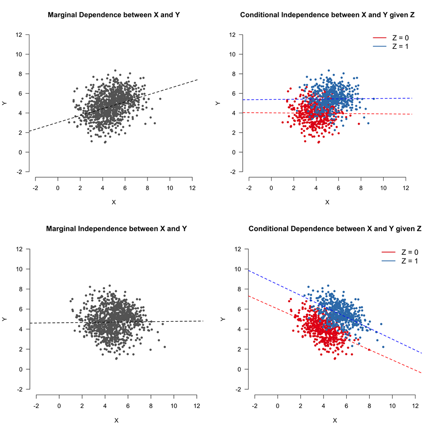
In the case of a chain, \(X\) and \(Y\) will be marginally dependent3, meaning that we should expect the correlation between \(X\) and \(Y\) to be non-zero if we do not adjust for \(Z\). However, adjusting for \(Z\) will make \(X\) and \(Y\) (conditionally) independent. In other words, once we know the value of \(Z\), \(X\) adds no useful information for understanding \(Y\). Using the independence symbol, \(\perp\!\!\!\perp\), we can represent these two findings as: \(X \not\!\perp\!\!\!\perp Y\) (\(X\) and \(Y\) are not independent) and \(X \perp\!\!\!\perp Y | Z\) (\(X\) and \(Y\) are independent if we condition on \(Z\)). The top panels of Figure 7.2 provide an illustrative example when \(Z\) is a binary variable.
Similarly, in the case of a fork or common cause, \(X\) and \(Y\) will be marginally correlated, but \(X\) and \(Y\) will be independent if we condition on \(Z\). Thus, a common cause will result in a spurious correlation between two unrelated variables (e.g., ice cream sales and number of severe sun burns; Figure 7.3) unless we condition on their common cause. This is a classic example used to highlight the impact of a confounding variable, \(Z\) (summer temperature).

One might get the impression, based on the above example and simple discussions of confounding variables in introductory statistics courses, that it is always best to include or adjust for other variables when fitting regression models. However, we can also create a spurious correlation by conditioning on a collider variable in an inverted fork. Specifically, if \(X \leftarrow Z \rightarrow Y\), then \(X\) and \(Y\) will be independent unless we condition on \(Z\) (i.e., \(X \perp\!\!\!\perp Y\), but \(X \not\!\perp\!\!\!\perp Y |Z\); see bottom row of panels in Figure 7.2). In essence, knowing \(X\) tells us nothing about \(Y\), that is, unless we are also given information about \(Z\). Once we have information about \(Z\), then knowing something about \(X\) gives us additional insights into likely values of \(Y\).
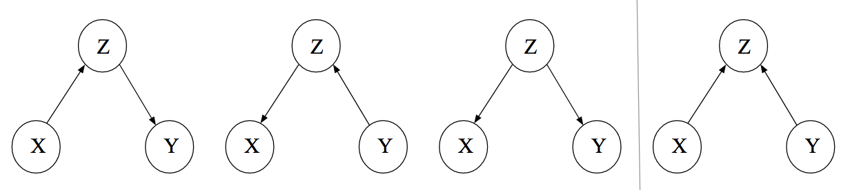
In summary, there are multiple DAGs that we could consider as representations of the causal connections between the variables \(X, Y\) and \(Z\) (Figure 7.4). The three DAGs on the left all result in the same set of (conditional) dependencies: \(X \not\!\perp\!\!\!\perp Y\), but \(X \perp\!\!\!\perp Y |Z\). Thus, it would be impossible to distinguish among them based on associations alone. The remaining DAG, where \(Z\) is a collider, results in the opposite set of (conditional) dependencies \(X \perp\!\!\!\perp Y\), but \(X \not\!\perp\!\!\!\perp Y |Z\).
7.3.1 Collider bias
Although the bias caused by confounding variables (e.g., a common cause) is well known, many readers may be surprised to hear that a spurious correlation can be created when we adjust for a variable. Thus, we will demonstrate this issue with a simple simulation example. Consider a survey of students at the University of Minnesota, where students are asked whether they are taking one or more classes on the St. Paul campus (\(Z_i = 1\) if yes and 0 otherwise), their level of interest in food science and nutrition \((X\) on a 10-point scale) and how many days they spent fishing in the past 3 years (\(Y\)). Because the St. Paul campus hosts the Department of Food Science and Nutrition and the Department of Fisheries, Wildlife, and Conservation Biology, we might expect students with high values of \(X\) or high values of \(Y\) to be taking one or more courses on the St. Paul campus. It is also conceivable that \(X\) and \(Y\) would be marginally independent (i.e., there is no causal connection between a person’s interest in nutrition \(X\) and how often they went fishing \(Y\)). We simulate data reflecting these assumptions4:
- We generate 10,000 values of \(X\) from a uniform distribution between 0 and 10.
- We generate 10,000 values of \(Y\), independent of \(X\), using a Poisson distribution with mean, \(\lambda\), equal to 4.
- We determine the probability that each student is taking a class on the St. Paul campus, \(p_i\), using:
\[p_i = \frac{exp(-5 + 2X + 2Y )}{1+exp(-5 + 2X + 2Y )}\]
When \(X\) and \(Y\) are both 0, \(p_i\) will equal 0.007; \(p_i\) will increase as either \(X\) or \(Y\) increases. Thus, students that are really interested in nutrition and students that really like to fish are both likely to be taking classes on the St. Paul campus. Lastly, we generate \(Z\) for each student using \(p_i\) and a Bernoulli distribution (equivalent to flipping a coin with probability \(p_i\) of a student taking one or more classes on the St. Paul campus).
# Set seed of random number generator
set.seed(1040)
# number of students
n <- 10000
# Generate X = interest in nutrition and food science
x <- runif(n, 0, 10)
# Generate number of days fishing
y <- rpois(n, lambda=4)
# Generate whether students are taking classes on St. Paul campus
p <- exp(-5 + 2*x + 2*y)/(1+exp(-5 + 2*x + 2*y))
z <- rbinom(n, 1, prob=p)
We then explore marginal and conditional relationships between \(X\) and \(Y\) by fitting regression models with and without \(Z\) (Table 7.1). We see that the coefficient for \(X\) is near 0 and not statistically significant when we exclude \(Z\) from the model (p = 0.535). This result is not surprising, given that we generated \(X\) and \(Y\) independently. However, \(X\) becomes negatively correlated with \(Y\) (and statistically significant) once we include \(Z\). Thus, including the predictor \(Z\) creates a spurious negative correlation between students’ interest in fishing and their interest in nutrition (implying that liking one spurs dislike of the other), a phenomenon often referred to as collider bias.
mod1 <- lm(y ~ x)
mod2 <- lm(y ~ x + z)| Parameter | Model 1 | Model 2 |
|---|---|---|
| (Intercept) | 3.970 (<0.001) | 1.457 (<0.001) |
| x | 0.004 (0.535) | -0.036 (<0.001) |
| z | 2.800 (<0.001) |
Importantly, collider bias can also occur if we restrict the study population using information in the collider variable, \(Z\) (Cole et al. 2010). For example, we also find that interest in nutrition and fishing are negatively correlated if we restrict ourselves to the population of students taking classes on the St. Paul campus:
collider.dat<-data.frame(x=x, y=y, z=z)
summary(lm(y ~ x, data=subset(collider.dat, z==1)))
Call:
lm(formula = y ~ x, data = subset(collider.dat, z == 1))

Residuals:
    Min      1Q  Median      3Q     Max
-4.1936 -1.2010 -0.1128  1.0351  9.1015

Coefficients:
             Estimate Std. Error t value Pr(>|t|)
(Intercept)  4.251386   0.041596 102.208  < 2e-16 ***
x           -0.035381   0.007101  -4.982 6.39e-07 ***
---
Signif. codes:  0 '***' 0.001 '**' 0.01 '*' 0.05 '.' 0.1 ' ' 1

Residual standard error: 1.985 on 9701 degrees of freedom
Multiple R-squared:  0.002553,  Adjusted R-squared:  0.00245
F-statistic: 24.83 on 1 and 9701 DF,  p-value: 6.386e-07
In essence, an interest in nutrition or an interest in fishing might lead someone to be represented in the study population of students on the St. Paul campus. Those students that end up in St. Paul due to their high interest in fishing likely have an average (or slightly-below average) level of interest in nutrition (assuming that interest in fishing and nutrition are independent in the full population of students). Similarly, students studying nutrition likely have an average to slightly below average level of interest in fishing. When we combine these two sets of students (students studying nutrition and students studying fisheries, wildlife, or conservation biology), we end up with a negative association between interest in fishing and interest in nutrition in the study population.
Similar concerns have been raised when analyzing data from hospitalized patients. As one example, Sackett (1979) found an association between locomotor disease and respiratory disease in hospitalized patients but not in the larger population. This result could be explained by a DAG in which hospitalization serves as a collider variable (Figure 7.5).

The importance of collider bias has also been recently highlighted in the context of occupancy models (MacKenzie et al. 2017), which are widely used in ecology. Using a simulation study, Stewart et al. (2023) showed that estimates of effect sizes associated with covariates influencing occupancy probabilities were biased when collider variables were considered for inclusion and information criterion (AIC and BIC; see Chapter 8) were used to select an appropriate model.
7.4 d-separation
We can use these same 3 basic rules to help determine, in larger causal networks, whether variables \(X\) and \(Y\) are independent after potentially conditioning on a set of other variables, \(Z\). However, we must consider all paths connecting \(X\) and \(Y\). We will refer to paths connecting variables as being either “open/correlating” or “closed/blocked”. If you forget the 3 basic rules, it can often help to think of flowing electricity when determining if a path is open or closed (if you can get from \(X\) to \(Y\), starting anywhere in the network then the path is open).
- chain: \(X \rightarrow Z \rightarrow Y\): if we add electricity to \(X\), it will flow to \(Y\). Thus, the pathway is open unless we include \(Z\) which will “block” the path.
- fork: \(X \leftarrow Z \rightarrow Y\): if we add electricity to \(Z\), it will flow to both \(X\) and \(Y\). Thus, the pathway between \(X\) and \(Y\) is open unless we include (i.e., condition on) \(Z\) which will block this path.
- inverted fork: \(X \rightarrow Z \leftarrow Y\): if we add electricity to either \(X\) or \(Y\) it will flow to \(Z\) and get stuck. If we add electricity to \(Z\) it will remain there. Thus, there is no way to connect \(X\) and \(Y\) unless we condition on \(Z\), which will open the pathway. It turns out, that conditioning on any of the descendants of \(Z\) will also open this pathway (Glymour et al. 2016). A descendant of \(Z\) is any variable that has an arrow (or set of arrows) that lead from \(Z\) into that variable.
Let’s now consider a more complicated causal network Figure 7.6.
To determine if two variables are dependent after conditioning on one or more variables, we will use the following steps:
- Write down all paths connecting the two variables.
- Determine if any of the paths are open/correlating. If any of the paths are open, then the two variables will be dependent. If all of the paths are blocked, then the two variables will be (conditionally) independent. When this occurs, we say that the variables are d-separated by the set of conditioning variables.
Let’s consider variables \(X\) and \(Y\) in Figure 7.6. There are two paths connecting these variables:
- \(X \rightarrow Z \rightarrow Y\)
- \(X \rightarrow W \leftarrow Y\)
The first path is a chain and is correlating (unless we condition on \(Z\)). The second path is an inverted fork and will be closed (unless we condition on \(W\) or its descendant \(U\)). Thus, we can infer the following set of conditional (in)dependencies:
- \(X \not\!\perp\!\!\!\perp Y\) (due to the first path being open)
- \(X \perp\!\!\!\perp Y | Z\) (conditioning on \(Z\) will close this open path)
- \(X \not\!\perp\!\!\!\perp Y |Z, W\) (conditioning on \(Z\) will close the first path, but conditioning on \(W\) will open up the second path)
- \(X \not\!\perp\!\!\!\perp Y |Z, U\) (conditioning on \(Z\) will close the first path, but conditioning on \(U\), which is a descendant of the collider \(W\), will open up the second path)
We can use functions in the ggm package to confirm these results (Marchetti et al. 2020). We begin by constructing the DAG using the DAG function to capture all arrows flowing into our variables:
library(ggm)
dag1<-DAG(W ~ X + Y,
          Z ~ X,
          Y ~ Z,
          V ~ Y,
          U ~ W)
We can then use the dSep function to test whether two variables \(X\) and \(Y\) (first and second arguments of the dSep function) are d-separated after conditioning on one or more variables (cond argument). Here, we confirm the 4 results from before:
dSep(dag1, first = "X", second= "Y", cond=NULL) [1] FALSEdSep(dag1, first = "X", second= "Y", cond="Z") [1] TRUEdSep(dag1, first = "X", second= "Y", cond=c("Z","W"))[1] FALSEdSep(dag1, first = "X", second= "Y", cond=c("Z","U"))[1] FALSE7.5 Estimating causal effects (direct, indirect, and total effects)
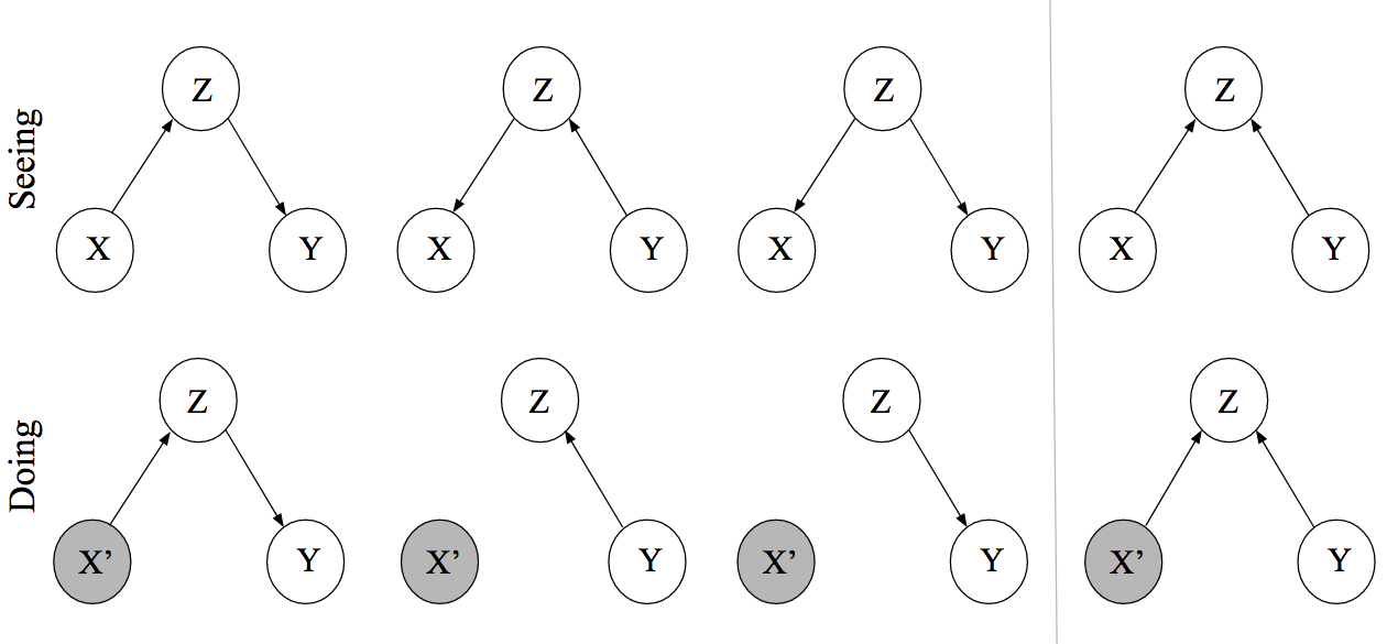
As was mentioned in the introduction to this section, when we want to intervene in a system, we often find that there are both direct and indirect effects on other variables. Formal methods have been developed (e.g., do calculus for calculating effects of interventions; Pearl et al. 2016; Dablander 2020). Although we will not go into detail about these methods here, it is useful to recognize that when we intervene in a system and set \(X = x\), this will effectively eliminate all connections flowing into \(X\). Consider all possible systems connecting variables \(X\), \(Y\), and \(Z\) (Figure 7.7). Setting \(X=x\) will have no effect on \(Y\) in the second, third, or fourth cases, since there are no directed paths connecting \(X\) to \(Y\) in these DAGS. This basic understanding underlies the mathematics behind quantifying the effects of interventions. For more details, we refer to Pearl et al. (2016) and Dablander (2020).
We can also consider how we can use DAGs to determine whether to include or exclude a variable from a regression model depending on whether we are interested in estimating a direct effect or total (sum of direct and indirect) effect. Let’s start by considering two examples from Pearl et al. (2016) and Dablander (2020) (Figure 7.8). Panel A depicts a situation in which a treatment (\(T\)) has, on average, a positive effect on patient’s response (\(R\)). A patient’s response will also depend on their sex (\(S\)). Lastly, the sex of the patient influences whether or not they will be treated. If we want to estimate the effect of the treatment, represented by \(T \rightarrow R\), we need to determine whether or not to adjust for sex.
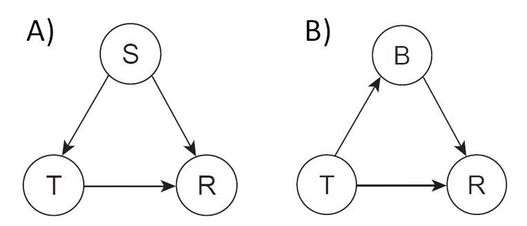
Let’s start by writing down all paths that connect \(T\) to \(R\):
- \(T \rightarrow R\)
- \(T \leftarrow S \rightarrow R\)
When fitting a regression model, we want the coefficient for \(T\) to reflect the causal effect (i.e., the first path). However, the second path will also be correlating due to the common cause \(S\). If we do not block this path, our coefficient for \(T\) will reflect associations arising from both of these paths. Thus, in this situation, we would want to include \(S\) in our regression model when estimating the effect of \(T\) on \(R\).
Now, let’s consider a second example where the treatment has both a direct effect on the response and an indirect effect through a variable \(B\) (Panel B in Figure 7.8). For example, a drug might have a direct effect on a patients recovery but also an indirect effect by increasing the patient’s blood pressure. We again have two paths that connect \(T\) and \(R\):
- \(T \rightarrow R\)
- \(T \rightarrow B \rightarrow R\)
Again, both of these paths are correlating. If we fit a model that includes only \(T\), then the coefficient for \(T\) will reflect both its direct and indirect effects on \(R\). Thus, if our interest is in knowing the overall (total) effect of the treatment on the patient’s response, we would not want to include \(B\) as it would block the second path. On the other hand, if we wanted to estimate the direct effect of \(T\) on \(R\), then we would want to block this path and include \(B\) in our model.
More generally, when we want to estimate a causal effect of \(X\) on \(Y\), we need to consider the backdoor criterion (Pearl et al. 2016). Specifically, we will need to
- Block all spurious (non-causal) paths between \(X\) and \(Y\)
- Leave all directed paths from \(X\) to \(Y\) unblocked (i.e., do not include mediator variables on the path between \(X\) and \(Y\)), and
- Make sure not to create spurious correlations by including colliders that connect \(X\) to \(Y\)
Consider again Figure 7.6 (shown again, below). If we want to calculate the causal effect of \(Z\) on \(U\), we can begin by writing down all paths connecting the two variables.
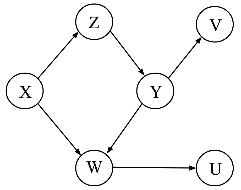
- \(Z \rightarrow Y \rightarrow W \rightarrow U\)
- \(Z \leftarrow X \rightarrow W \rightarrow U\)
The first path is our directed path connecting \(Z\) to \(U\) (and our effect of interest). The second is a correlating path due to a common cause, \(X\). To satisfy the backdoor criterion, we need to 1) block the second path (e.g., by including \(X\)), and 2) make sure not to include \(Y\) or \(W\) as these would block our path of interest. See Laubach et al. (2021) and Cinelli et al. (2024) for additional examples and discussion regarding how DAGs should be used to choose appropriate predictor variables when estimating causal effects.
7.6 Some (summary) comments
We have seen how simple causal diagrams can help with understanding if and when we should include variables in regression models. Hopefully, you will keep these ideas in mind when learning about other less thoughtful, data-driven methods for choosing a model (Chapter 8). In particular, it is important to recognize that a “best fitting” model may not be the most appropriate one for addressing your particular research question, and in fact, it can be misleading (Luque-Fernandez et al. 2019; Stewart et al. 2023; Arif and MacNeil 2022; Addicott et al. 2022).
One challenge with implementing causal inference methods is they rely heavily on assumptions (i.e., an assumed graph capturing causal relationships between variables in the system). And although it is sometimes possible to work backwards, using the set of observed statistical independencies in the data to suggest or rule out possible causal models, multiple models can lead to the same set of statistical independencies (Shipley 2002). In these cases, experimentation can prove critical for distinguishing between competing hypotheses.
Lastly, it is important to consider multiple lines of evidence when evaluating the strength of evidence for causal effects. In that spirit, I end this section with Sir Austin Bradford Hill’s5 suggested criteria needed to establish likely causation (the list below is taken verbatim from https://bigdata-madesimple.com/how-to-tell-if-correlation-implies-causation/):
- Strength: A relationship is more likely to be causal if the correlation coefficient is large and statistically significant.
- Consistency: A relationship is more likely to be causal if it can be replicated.
- Specificity: A relationship is more likely to be causal if there is no other likely explanation.
- Temporality: A relationship is more likely to be causal if the effect always occurs after the cause.
- Gradient: A relationship is more likely to be causal if a greater exposure to the suspected cause leads to a greater effect.
- Plausibility: A relationship is more likely to be causal if there is a plausible mechanism between the cause and the effect
- Coherence: A relationship is more likely to be causal if it is compatible with related facts and theories.
- Experiment: A relationship is more likely to be causal if it can be verified experimentally.
- Analogy: A relationship is more likely to be causal if there are proven relationships between similar causes and effects.
7.7 References
Addicott, Ethan T, Eli P Fenichel, Mark A Bradford, Malin L Pinsky, and Stephen A Wood. 2022. “Toward an Improved Understanding of Causation in the Ecological Sciences.” Frontiers in Ecology and the Environment 20 (8): 474–80.
Arif, Suchinta, and M Aaron MacNeil. 2022. “Predictive Models Aren’t for Causal Inference.” Ecology Letters 25 (8): 1741–45.
Cinelli, Carlos, Andrew Forney, and Judea Pearl. 2024. “A Crash Course in Good and Bad Controls.” Sociological Methods & Research 53 (3): 1071–104.
Cole, Stephen R, Robert W Platt, Enrique F Schisterman, et al. 2010. “Illustrating Bias Due to Conditioning on a Collider.” International Journal of Epidemiology 39 (2): 417–20.
Dablander, Fabian. 2020. An Introduction to Causal Inference. .
Glymour, Madelyn, Judea Pearl, and Nicholas P Jewell. 2016. Causal Inference in Statistics: A Primer. John Wiley & Sons.
Kaplan, D. 2009. Statistical Modeling: A Fresh Approach. CreateSpace Independent Publishing Platform. https://books.google.com/books?id=xphtQgAACAAJ.
Laubach, Zachary M, Eleanor J Murray, Kim L Hoke, Rebecca J Safran, and Wei Perng. 2021. “A Biologist’s Guide to Model Selection and Causal Inference.” Proceedings of the Royal Society B 288 (1943): 20202815.
Lock, Robin H, Patti Frazer Lock, Kari Lock Morgan, Eric F Lock, and Dennis F Lock. 2020. Statistics: Unlocking the Power of Data. John Wiley & Sons.
Luque-Fernandez, Miguel Angel, Michael Schomaker, Daniel Redondo-Sanchez, Maria Jose Sanchez Perez, Anand Vaidya, and Mireille E Schnitzer. 2019. “Educational Note: Paradoxical Collider Effect in the Analysis of Non-Communicable Disease Epidemiological Data: A Reproducible Illustration and Web Application.” International Journal of Epidemiology 48 (2): 640–53.
MacKenzie, Darryl I, James D Nichols, J Andrew Royle, Kenneth H Pollock, Larissa Bailey, and James E Hines. 2017. Occupancy Estimation and Modeling: Inferring Patterns and Dynamics of Species Occurrence. Elsevier.
Marchetti, Giovanni M., Mathias Drton, and Kayvan Sadeghi. 2020. Ggm: Graphical Markov Models with Mixed Graphs. https://CRAN.R-project.org/package=ggm.
Pearl, J. 2000. Causality: Models, Reasoning, and Inference. Cambridge University Press.
Pearl, Judea. 1995. “Causal Diagrams for Empirical Research.” Biometrika 82 (4): 669–88. https://doi.org/10.1093/biomet/82.4.669.
Pearl, Judea, Madelyn Glymour, and Nicholas P Jewell. 2016. Causal Inference in Statistics: A Primer. John Wiley & Sons.
Pearl, Judea, and Dana Mackenzie. 2018. The Book of Why: The New Science of Cause and Effect. Basic books.
Rossman, Allan J. 1994. “Televisions, Physicians, and Life Expectancy.” Journal of Statistics Education 2 (2).
Sackett, David L. 1979. “Bias in Analytic Research.” In The Case-Control Study Consensus and Controversy. Elsevier.
Shipley, B. 2002. Cause and Correlation in Biology: A User’s Guide to Path Analysis, Structural Equations and Causal Inference. Cambridge University Press.
Stewart, Peter S, Philip A Stephens, Russell A Hill, Mark J Whittingham, and Wayne Dawson. 2023. “Model Selection in Occupancy Models: Inference Versus Prediction.” Ecology 104 (3): e3942.
Wright, Sewall. 1921. “Correlation and Causation.” Journal of Agricultural Research 20: 557–85.
https://www.realtree.com/deer-hunting/articles/earn-a-buck-was-it-the-greatest-deer-management-tool↩︎
In most years, my students discover Tyler Vigen’s web site (http://tylervigen.com/spurious-correlations), which offers many other silly examples of ridiculously strong correlations over time between variables that do not themselves share a causal relationship.↩︎
Marginal here refers to the unconditional relationship between \(X\) and \(Y\) rather than the strength of this relationship.↩︎
We will learn more about the distributions used to simulate data when we get to Chapter 9.↩︎
Sir Austin Bradford Hill was a famous British medical statistician.↩︎