This book is in Open Review. I want your feedback to make the book better for you and other readers. To add your annotation, select some text and then click the on the pop-up menu. To see the annotations of others, click the in the upper right hand corner of the page

9  Introduction to probability distributions

Learning objectives

1. Understand and be able to work with basic rules of probability. We will need these rules to understand Bayes Theorem, which is fundamental to Bayesian statistics.

2. Gain a basic familiarity with concepts related to mathematical statistics (e.g., random variables, probability mass and density functions, expected value, variance, conditional and marginal probability distributions).

3. Understand how to work with different statistical distributions in R.

4. Understand the role of random variables and common statistical distributions in formulating modern statistical regression models.

5. Be able to choose an appropriate statistical distribution for modeling your data.

9.1 Statistical distributions and regression

Up until now, our focus has been on linear regression models, which can be represented as:

$$\begin{array}{r}{Y}_i={\beta }_0+X_i{\beta }_1+{ϵ}_i\\ {ϵ}_i\sim N(0,{\sigma }^2)\end{array}$$ or

$$Y_i\sim N({\beta }_0+X_i{\beta }_1,{\sigma }^2)$$ or

$$Y_i\sim N({\mu }_i,{\sigma }^2)$$ $$\begin{array}{}\text{(9.1)}& {\mu }_i={\beta }_0+X_i{\beta }_1\end{array}$$

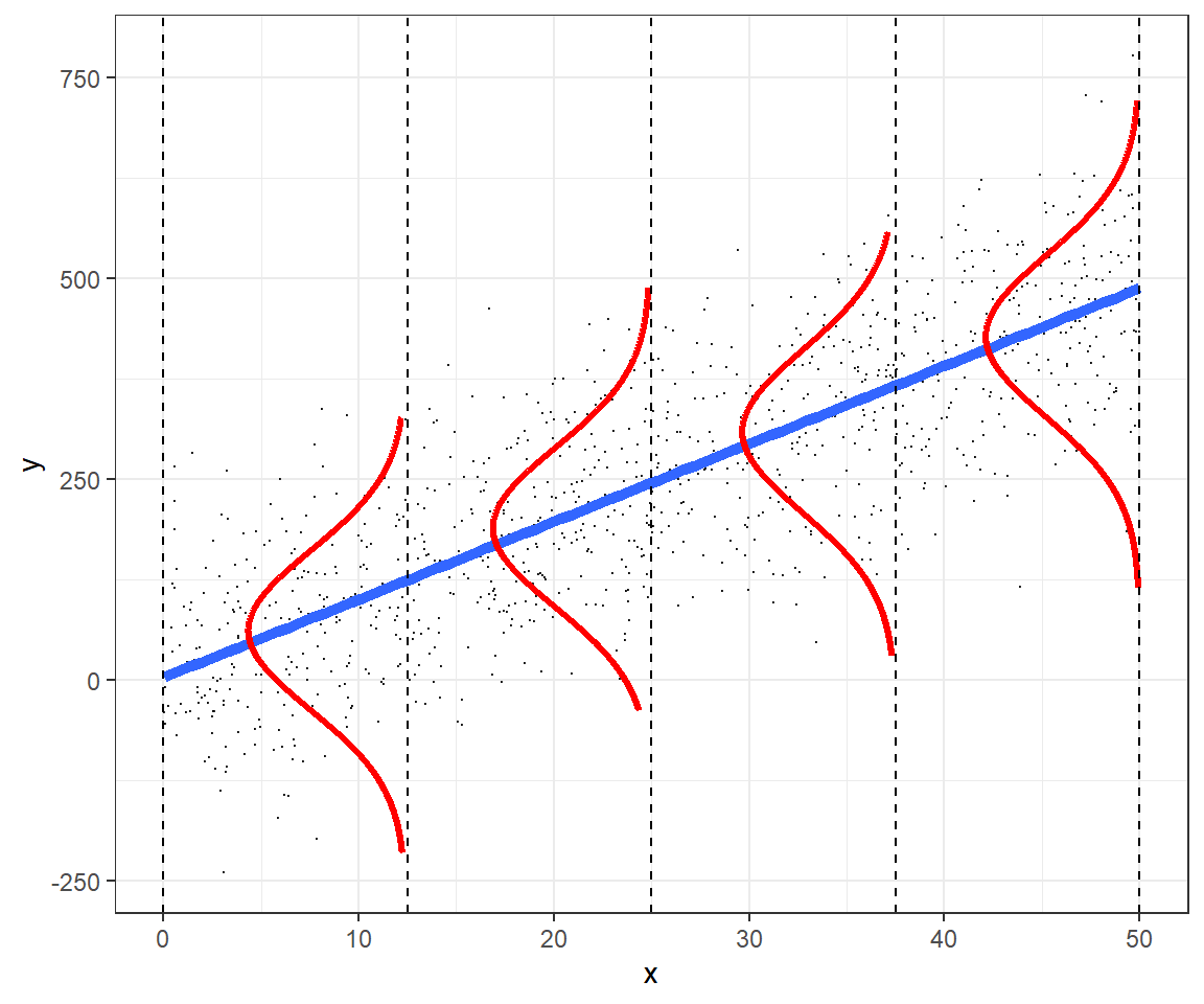
Moving forward, we are going to use the last formulation to emphasize the role of the Normal distribution as our data-generating model. This formulation allows us to easily see that we are:

1. Modeling the mean, ${\mu }_i$, of the Normal distribution as a linear combination of our explanatory variables; GLS models (Chapter 5) also allow us to model ${\sigma }_i$ as a function of explanatory variables.

• The Normal distribution describes the variability of the observations about ${\mu }_i$.

Figure 9.1: The role of the Normal distribution as a data-generating model. This figure was produced using modified code from an answer on stackoverflow by Roback and Legler (2021) (https://bookdown.org/roback/bookdown-bysh/).

The Normal distribution has several characteristics that make it a poor data generating model for certain types of data (e.g., count or binary data):

• the distribution is bell-shaped and symmetric
• observations can take on any value between $-\mathrm{\infty }$ and $\mathrm{\infty }$

In this chapter, we will learn about other statistical distributions and ways to work with them in R. Along the way, we will learn about discrete and continuous random variables and their associated probability mass functions (discrete random variables) and probability density functions (continuous random variables). We will also learn a few basic probability rules that can be useful for understanding Bayesian methods and for constructing models using conditional probabilities (e.g., occupancy models; MacKenzie et al. 2017).

9.2 Probability rules

We will begin by highlighting a few important probability rules that we will occasionally refer back to:

1. Multiplicative rule: $P(A\text{ and }B)=P(A)P(B\mid A)=P(B)P(A\mid B)$
2. Union: $P(A\text{ or }B)=P(A)+P(B)-P(A\text{ and }B)$
3. Complement rule: $P(\text{not }A)=1-P(A)$
4. Conditional probability rule: $P(A\mid B)=\frac{P(A\text{ and }B)}{P(B)}$

If you forget these rules, it is often helpful to create a visualization using a Venn diagram (i.e., an illustration with potentially overlapping circles representing different events). For example, consider the Venn diagram representing numbers between 1 and 10 along with whether the numbers are prime and whether they are even (Figure 9.2).

Figure 9.2: Venn diagram with even and prime numbers from 1 to 10. Guy vandegrift / Wikimedia Commons / CC-BY-SA 4.0 International.

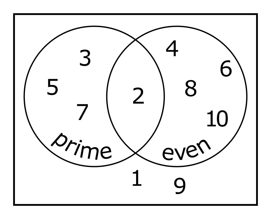
Let $A$ represent the set of prime numbers and $B$ represent the set even numbers. We see that $P(A\text{ and }B)$ is determined by the intersection of the two circles and is equal to 1/10 (i.e., there is only one number, 2, in the intersection out of ten possible numbers). To understand the Union rule, we can consider that $P(A)=4/10$ and $P(B)=5/10$. To determine $P(A\text{ or }B)$, we can by sum these two probabilities, but then we need to subtract $P(A\text{ and }B)$. Otherwise, we would be including the number 2 twice.

It is also helpful to know of two special cases having to do with mutually exclusive or independent events. If events A and B are mutually exclusive (meaning that they both cannot happen), then:

• $P(A\text{ or }B)=P(A)+P(B)$
• $P(A\text{ and }B)=0$

If events A and B are independent:

• $P(A\mid B)=P(A)$ (intuitively, if A and B are independent, knowing that event B happened does not change the probability that event A happened)
• $P(A\text{ and }B)=P(A)P(B)$ (we will use this rule when we construct likelihoods)

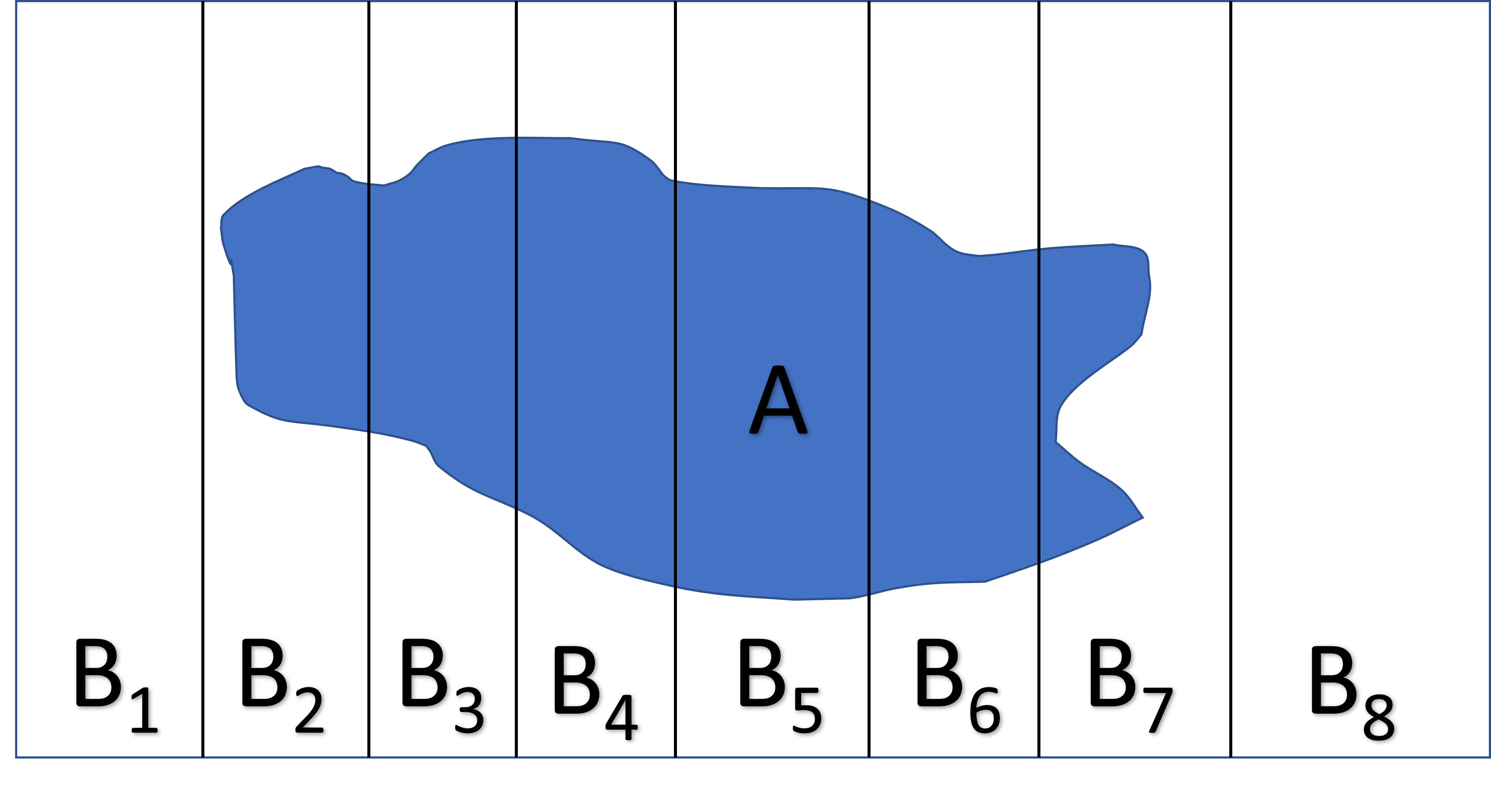
Lastly, it will be helpful to know the Law of Total Probability (Figure 9.3). If we partition the sample space into a set of $k$ mutually exclusive events, $B_1,B_2,\dots ,B_k$, that together make up all possibilities, then:

$$P(A)=\sum _{i=1}^{k}P(A|B_i)P(B_i)$$

Figure 9.3: The total law of probability, $P(A)=\sum _{i=1}^{k}P(A|B_i)P(B_i)$, can be understood by partitioning the sample space into a discrete number of mutually exclusive events that together make up all possibilities.

A special case of the total law of probability is:

$$P(A)=P(A\text{ and }B)+P(A\text{ and }(\text{not }B))$$

Lastly, we can combine several of these probability rules to form Bayes Theorem:

$$P(A\mid B)=\frac{P(A\text{ and }B)}{P(B)}$$ $$=\frac{P(B\mid A)P(A)}{P(B\text{ and }A)+P(B\text{ and not }A)}$$ $$\begin{array}{}\text{(9.2)}& =\frac{P(B\mid A)P(A)}{P(B\mid A)P(A)+P(B\mid \text{not }A)P(\text{not }A)}\end{array}$$ \end{gather}

We can also write Bayes rule more generally as:

$$\begin{array}{}\text{(9.3)}& P(A\mid B)=\frac{P(B\mid A)P(A)}{\sum _{i=1}^{k}P(B\mid A_i)P(A_i)}\end{array}$$

9.2.1 Application of Bayes theorem to diagnostic screening tests

Bayes theorem is the foundation of Bayesian statistics, but it is also often used for frequentist inference, for example, to understand results of various diagnostic tests for which we often have poor intuition (Bramwell, West, and Salmon 2006). As an example, consider the following question posed by Bramwell, West, and Salmon (2006):

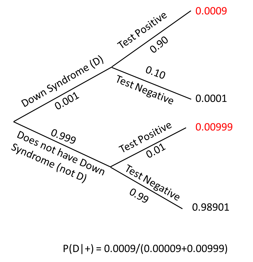
The serum test screens pregnant women for babies with Down’s syndrome. The test is a very good one, but not perfect. Roughly 1% of babies have Down’s syndrome. If the baby has Down’s syndrome, there is a 90% chance that the result will be positive. If the baby is unaffected, there is still a 1% chance that the result will be positive. A pregnant woman has been tested and the result is positive. What is the chance that her baby actually has Down’s syndrome?

The answer, using the information above, is $\approx 48\mathrm{\%}$. Surprised? You are not alone – Bramwell, West, and Salmon (2006) found that only 34% of obstetricians, 0% of midwives, and 9% of pregnant females arrived at this correct answer (and many of these participants benefited from an alternative presentation in terms of frequencies); See also Weber, Binder, and Krauss (2018) for a similar investigation.

The 1% prevalence rate assumed by Bramwell, West, and Salmon (2006) is close to what the CDC reports for women that are 40 years old or older. The prevalence rate in the general population is actually much lower (closer to 0.1%). As a result, the probability that a baby has Down’s syndrome given that a younger mother receives a positive test is actually much lower than 48%. Let’s repeat the analysis with the lower prevalence rate of 0.1%.

Let:

• $P(D)$ = the probability that a randomly chosen newborn will have Down’s syndrome = 0.001.
• $P(+|D)$ = the probability of a positive test, given the baby has Down’s syndrome = 0.90.
• $P(+|\text{ not }D)$ = the probability of a positive test given the baby does not have Down’s syndrome = 0.01

Our goal is to use Bayes’ theorem to calculate the probability a baby will have Down’s syndrome given that the mother tests positive, $P(D|+)$. We can figure out the different pieces of information we need by writing down Bayes’ rule in the context of our diagnostic testing example:

$$\begin{array}{}\text{(9.4)}& P(D|+)=\frac{P(+\mid D)P(D)}{P(+\mid D)P(D)+P(+\mid \text{ not }D)P(\text{not }D)}\end{array}$$

Thus, we need the following:

• $P(\text{not }D)=1-P(D)$ (using the complementary rule) = 0.999
• $P(-|D)=1-P(+|D)$ = 0.10

Plugging these values in to Equation 9.4, we get:

$$\begin{array}{}\text{(9.5)}& P(D|+)=\frac{(0.90)(0.001)}{(0.90)(0.001)+(0.01)(0.999)}=0.083\text{ or }\approx 8\mathrm{\%}\end{array}$$

Although this is an order of magnitude larger than the prevalence rate in the population, the probability of the child having Down’s is still low – only 8% – even with a positive test! I remember working through the math when my wife was first pregnant with our oldest child, Zoe, and concluding that we had no interest in the diagnostic test. Many diagnostic tests suffer a similar same fate when prevalence rates in the population are really low.

Figure 9.4: As highlighted by this comic, many diagnostic tests suffer from extremely high false positive rates due to low prevalence rates in the population. Image from https://xkcd.com/2545/. CC BY-NC 2.5

9.2.2 Bayes rule and problems with multiple testing

Another really useful application of Bayes rule is in understanding problems associated with conducting multiple null hypothesis tests, particularly when hypotheses do not have strong a priori support or when the tests have low power (i.e., probability of detecting an effect when one exists). Let’s consider a scenario in which we test 1000 hypotheses. Assume:

• 10% of the hypotheses are truly false, $P(H_0=true)=0.1$.
• We have an 80% chance of rejecting the hypothesis given that it is false, $\beta =P(Reject|H_0=false)=0.80$.
• We use an $\alpha =0.05$ to conduct all tests so that the probability of rejecting a hypothesis when it is true is 5%, $P(Reject|H_0=true)=0.05$.

Given these assumptions, we should expect to report a total of 125 significant findings, but 36% of these significant findings will be incorrect (i.e., rejections when the null hypothesis is true); 64% will be correct. We can use Bayes rule to verify this result. Let’s calculate the probability the null hypothesis is false, given that we rejected it:

$$\begin{array}{c}P(H_0=false|Reject)=\frac{P(Reject|H_0=false)P(H_0=false)}{P(Reject|H_0=false)P(H_0=false)+P(Reject|H_0=true)P(H_0=true)}\\ =\frac{(0.8)(0.1)}{(0.8)(0.1)+(0.05)(0.9)}=0.64\end{array}$$

Ioannidis (2005) used this framework to explain why studies that attempt to replicate research findings so often fail. The situation may be even worse in ecology, given that the power of most ecological studies is well below 80% and often closer to 20% (see Forstmeier, Wagenmakers, and Parker 2017 and references therein). If we repeat the above calculations but for studies with only 20% power, we find $P(H_0=false|Reject)$ is only around 0.30. I.e., the majority of the time that we think we are discovering something interesting, we are actually being misled.

9.3 Probability Trees

When working through compound probabilities (i.e., probabilities associated with 2 or more independent events), it can often be useful to draw a tree diagram that outlines all of the different possibilities calculated by repeatedly applying the conditional probability rule, $P(A\text{ and }B)=P(A)P(B|A)$. We show the tree diagram for the diagnostic testing problem below:

Figure 9.5: Probability tree for calculating the probability that a child will have Downs Syndrome given the mother tests positive. Probability trees represent all possible outcomes associated with multiple events using a branching process. Probabilities associated with each outcome can be determined by multiplying successive probabilites along each branch.

9.3.1 Just for fun: Monte Hall problem

Many of you may have seen a version of the Monte Hall problem before. One of the main reasons I like this problem is that, like the diagnostic testing problem, it can highlight how poor our intuition is at times when working with probabilities. The problem goes like this: suppose you are on a game show where the host asks you to choose from one of 3 doors. Behind one of the doors is a brand new car. Behind the other two are a goat. You are asked to choose a door (if you select the door with the car, you win the car). After you reveal your choice, the host opens one of the doors that you did not choose and shows you a goat. The game show host then asks whether you want to change your initial decision. If you are like most people, you will likely stick with your initial choice, thinking that you have a 50-50 chance of winning either way. But, it turns out that you increase your chances of winning by switching doors. If you switch, you have a 2/3 chance of winning versus 1/3 if you stick with your initial choice!

One way to understand this result is to construct a probability tree representing the initial event (choosing a door with or without a goat) and then the final outcome, conditional on your initial choice and whether you choose to change your decision or not after seeing the game show host reveal one of the 2 goats. If you initially chose a door with a goat, then you will end up with the car if you switch doors. If you initially chose the door with the car, then you will end up with a goat if you switch. The thing is, you are more likely to initially choose a door with a goat than the door with the car. So, in the end, you are best off switching doors once you can eliminate the door where the goat has been revealed.

Figure 9.6: Probability tree for the Monte Hall problem.

If this result is surprising to you, you are not alone. For a really interesting read that highlights just how many (mostly overconfident male) PhD scientists not only got this answer wrong, but also choose to publicly deride Marilyn vos Savant (better known for her “Ask Marilyn” column in Parade Magazine) for providing the correct answer see this aticle. You might also be interested in knowing that pigeons (Columba livia) have performed better than humans at solving the Monte Hall problem (Herbranson and Schroeder 2010)!

9.4 Sample space, random variables, probability distributions

In frequentist statistics, probabilities are defined in terms of frequencies of events. Specifically, the probability of event A, $P(A)$, is defined as the proportion of times the event would occur in an infinite set of random trials with the same underlying conditions. To define a probability distribution, we first need to define the sample space of all possible outcomes that could occur and a random variable that maps these events to a set of real numbers. We can then map the real numbers to probabilities using a probability distribution.

A key consideration is whether we are interested in modeling the distribution of a discrete or continuous random variable. Discrete variables take on a finite or countably infinite number of values¹. Examples include:

• age classes = (fawn, adult)
• the number of birds counted along a transect
• whether or not a moose calf survives its first year
• the number of species counted on a beach in the Netherlands

Continuous variables, by contrast, can take on any real number. Examples include:

• (lat, long) coordinates of species in an INaturalist database
• the age at which a randomly selected adult white-tailed deer dies
• mercury level (ppm) in a randomly chosen walleye from Lake Mille Lacs

9.4.1 Discrete random variables

Discrete random variables are easier to consider than continuous random variables because we can directly map events to probabilities. Let’s consider a specific example. Consider sampling 2 white-tailed deer for chronic wasting disease. Assume our 2 individuals are randomly chosen from a population where the prevalence rate of chronic wasting disease is $p$.

In this case, the possible events are: (-, -), (-, +), (+, -), (+, +). We could define a random variable, $Y$ = the number of positive tests. Then, our sample space for $Y$ = {0, 1, 2}. Note, it is customary to write random variables using capital letters ($Y$) and realizations of random variables using lower case letters ($y$). Thus, $Y$ would describe a random quantity (not yet observed) having a statistical distribution, whereas $y$ would describe a specific observed value of the random variable $Y$.

We next define a probability mass function, $f(y;p)$, that maps the sample space of $Y$ to probabilities (Table 9.1). When referring to probability mass or probability density functions that include one or more parameters, we will often use the notation, $f(variable;parameters)$ (here, $f(y;p)$). Sometimes I may forget to include the parameter(s) (or just get lazy) and use $f(y)$ instead.

Table 9.1: Probability distribution for the number of positive tests for chronic wasting disease in a random sample of 2 deer in a population with prevalence rate p.

Y	f
0	(1-p)(1-p)
1	2p(1-p)
2	$p^2$

These probabilities can be easily derived by noting the probability of a positive test is $p$, the probability of a negative test is $1-p$, and if events A and B are independent, then P(A and B) = P(A)P(B); see Section 9.2. This example is a special case of the binomial distribution with $n=2$, which we will learn more about in Section 9.10.2.

9.4.2 Continuous random variables

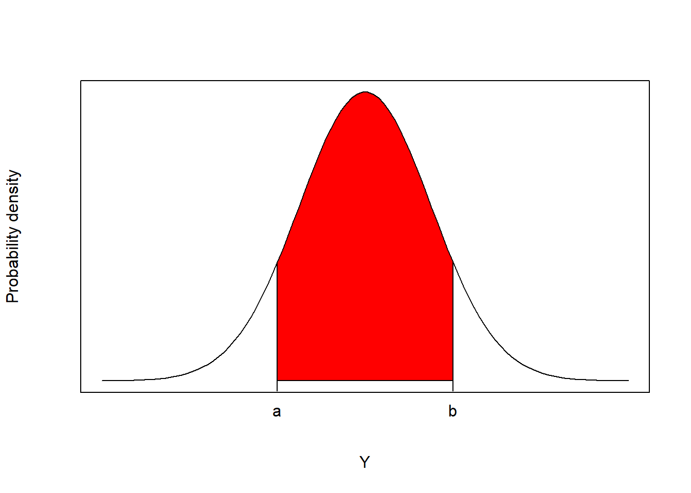
For continuous random variables, there are an infinite number of values that $Y$ can take on. Thus, we no longer assign probabilities to specific values of $Y$, but rather use probability density functions, $f(y;\theta )$, to determine the probability that $Y$ takes on a value within an interval $(a,b)$, $P(a\le Y\le b)$:

$$\begin{array}{}\text{(9.6)}& P(a\le Y\le b)={\int }_a^{b}f(y;\theta )dy\end{array}$$

You may recall from calculus that integrating $f(y;\theta )$ is equivalent to finding the area under the curve (Figure 9.7).

Figure 9.7: For continuous random variables, probabilities are defined as the areas under the curve of a probability density function.

A few other things to note about continuous random variables are:

• The probability associated with any point is 0; $P(Y=y)=0$ for all $y$. Thus, we can choose to write $P(a\le Y\le b)$ or equivalently, $P(a<Y<b)$.
• ${\int }_{\mathrm{\infty }}^{\mathrm{\infty }}f(y;\theta )=1$ (the total area under any probability density function is equal to 1).

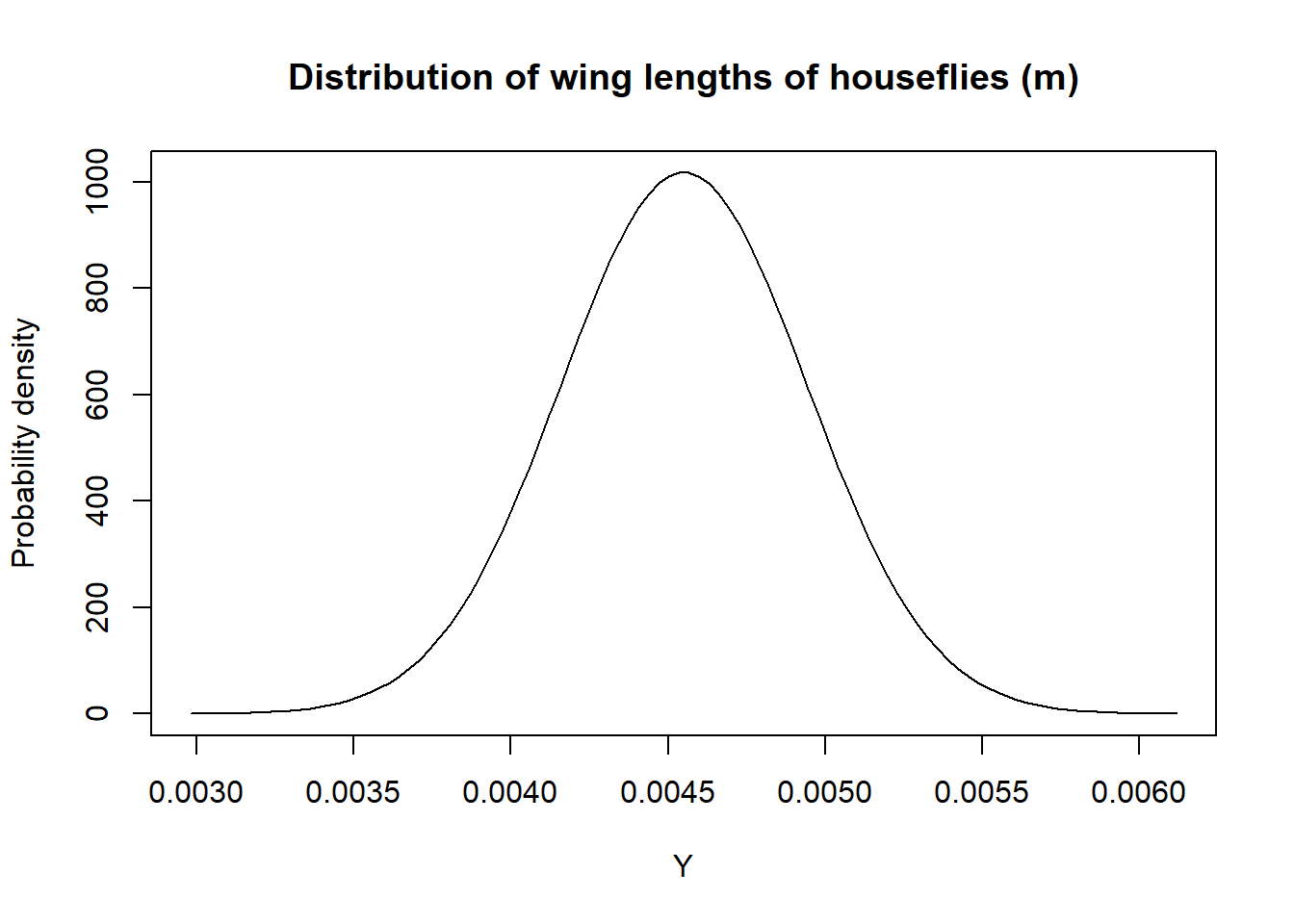
Also, note that unlike probability mass functions, probability density functions can take on values greater than 1. To understand why this must be the case, consider representing the distribution of wing-lengths of houseflies in meters using a Normal distribution with mean = 0.00455 m and standard deviation = 0.000392 m. The range of wing-lengths is much less than 1, so the probability density function must be much greater than 1 for many values of $Y$ to ensure that the total area under the curve is 1 (Figure 9.8).

Figure 9.8: Distribution of wing-lengths for common houseflies in meters.

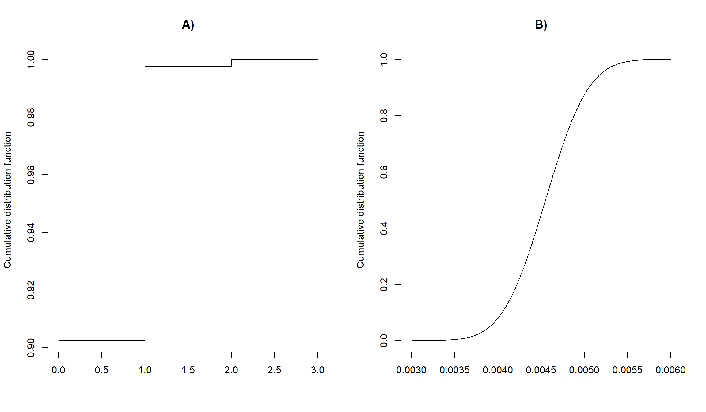
9.5 Cumulative distribution functions

We will often want to determine $F(Y)=P(Y\le a)$ or its complement, $1-P(Y\le a)=P(Y>a)$; $P(Y\le a)$ is called the cumulative distribution function (CDF). The CDF can be written as:

$$F(Y)=P(Y\le y)={\int }_{-\mathrm{\infty }}^{x}f(y;\theta )dy$$

The cumulative distribution functions for our chronic wasting disease example assuming $p=0.5$ and the housefly wing length example are depicted in (Figure 9.9). Note, that $F(-\mathrm{\infty })=0$ and $F(\mathrm{\infty })=1$ for all probability distributions.

Figure 9.9: Cumulative distribution functions for the chronic wasting disease example (binomial distribution) and the housefly example (Normal distribution).

9.6 Expected value and variance of a random variable

For Discrete random variables, we define the expected value and variance as:

• $E[Y]=\sum yf(y;\theta )$
• $Var[Y]=\sum (y-E[Y]{)}^{2}f(y;\theta )$

For continuous random variables, we define the expected value and variance as:

• $E[Y]={\int }_{-\mathrm{\infty }}^{\mathrm{\infty }}yf(y;\theta )dy$
• $Var[Y]={\int }_{-\mathrm{\infty }}^{\mathrm{\infty }}(y-E[Y]{)}^{2}f(y;\theta )dy$

The expected value gives the average value you would see if you generated a large number of random values from the probability distribution. Also, note that the standard deviation of a random variable is equal to $\sqrt{Var[Y]}$.

Example: Let’s calculate the mean and variance of our random variable describing the number of positive tests for chronic wasting disease when sampling 2 random deer:

$$E[Y]=0[(1-p{)}^2]+1[2p(1-p)]+2[p^2]=2p-2p^2+2p^2=2p$$ $$Var[Y]=(0-2p{)}^2[(1-p{)}^2]+(1-2p{)}^2[2p(1-p)]+(2-2p{)}^2[p^2]=2p(1-p)$$

Deriving the final expression for the variance requires a lot of algebra (but, can be simplified using online calculators – e.g., here). Note, it is often easier to derive the variance using an alternative formula:

• $Var[Y]=E[Y^2]-(E[Y]{)}^2$ where $E[Y^2]=\sum y^{2}f(y;\theta )$

If you were to take a mathematical statistics course, you would likely derive this alternative expression for the variance and also derive expressions for the mean and variance associated with several common probability distributions.

9.7 Expected value and variance of sums and products

We will often need to calculate the expected value or variance of a sum or product of random variables. For example, in Section 3.12, we needed to be able to determine the variance of a sum of regression parameter estimates when calculating the uncertainty associated with pairwise differences between means for different values of a categorical variable. Similarly, in Chapter 5, we needed to calculate the mean and variance for a linear combination of our regression parameters in order to plot $E[Y_i|X_i]$. Here, we state three useful results for the case of 2 random variables, $X$ and $Y$:

• $E[X+Y]=E[X]+E[Y]$
• $Var[X+Y]=Var[X]+Var[Y]+2Cov[X,Y]$
• If $X$ and $Y$ are independent, $E[XY]=E[X]E[Y]$

9.8 Joint, marginal, and conditional distributions

There are many situations where we may be interested in considering more than 1 random variable at a time. In these situations, we may consider:

• joint probability distributions describing probabilities associated with all random variables simultaneously.
• conditional distributions describing probabilities for one or more of the random variables, given a realization of the other random variables.
• marginal distributions describing the probability of one of the random variables, which can be determined by averaging over all possible values of the other random variables.

Again, these concepts are easiest to understand when modeling discrete random variables since we can use a joint probability mass function to assign probabilities directly to unique combinations of the values associated with the two random variables. Consider the following simple example with two random variables, $X$ and $Y$:

• $X$ takes on a value of 1 when a randomly chosen site is occupied by a species of interest and 0 otherwise
• $Y$ takes on a value of 1 when the species of interest is detected at a randomly chosen site and 0 otherwise

We will assume that the probability that a randomly chosen site is occupied by the species of interest is given by $\mathrm{\Psi }$. Thus, the probability mass function for $X$, $f_x(x)$ is given by:

• $f_x(0)=1-\mathrm{\Psi }$
• $f_x(1)=\mathrm{\Psi }$

We will further assume that the probability that a species is detected at a randomly chosen site is equal to $p$ if the site is occupied and 0 otherwise. Thus, the conditional probability mass function for $Y|X$ (“$Y$ given $X$”), $f_y(y|x)$, is given by:

• $f_y(0|x=0)=1$
• $f_y(1|x=0)=0$

when $X=0$ and

• $f_y(0|x=1)=1-p$
• $f_y(1|x=1)=p$

when $X=1$.

Joint distribution from a conditional and marginal distribution

We can derive the joint probability mass function for $(X,Y)$, $f_{x,y}(x,y)$, using the multiplicative probability rule: $f_{x,y}(x,y)=f_y(y|x)f_x(x)$:

• $f_{x,y}(0,0)=1-\mathrm{\Psi }$ (site is unoccupied and therefore the species is not detected)
• $f_{x,y}(0,1)=0$ (the site is unoccupied but the species is detected; equal to 0 when there are no false positives)
• $f_{x,y}(1,0)=\mathrm{\Psi }(1-p)$ (the site is occupied, but we do not detect the species)
• $f_{x,y}(1,1)=\mathrm{\Psi }p$ (the site is occupied, and we detect the species)

We can verify that this is a valid joint probability distribution by noting that $0\le f(x,y)\le 1$ for all values of $x$ and $y$, and $\sum _{(x,y)}f(x,y)=1-\mathrm{\Psi }+\mathrm{\Psi }(1-p)+\mathrm{\Psi }p=1$.

Marginal distribution from the joint distribution

We can derive the marginal probability mass function of $Y$, $f_y(y)$, using the total law of probability: $f_y(y)=\sum _x{f}_{x,y}(x,y)$:

• $f_y(0)=f_{x,y}(0,0)+f_{x,y}(1,0)=1-\mathrm{\Psi }+\mathrm{\Psi }(1-p)=1-\mathrm{\Psi }p$ (probability of not detecting the species)
• $f_y(1)=f_{x,y}(0,1)+f_{x,y}(1,1)=\mathrm{\Psi }p$ (probability of detecting the species)

Conditional distribution from the joint and marginal distribution

We can then derive the distribution of $X|Y$, $f_x(x|y)$, using the conditional probability rule: $f_x(x|y)=\frac{f_{x,y}(x,y)}{f_y(y)}$. When $Y$ = 0, we have:

• $f_x(0|y=0)=\frac{1-\mathrm{\Psi }}{1-\mathrm{\Psi }p}$
• $f_x(1|y=0)=\frac{\mathrm{\Psi }(1-p)}{1-\mathrm{\Psi }p}$

Importantly, this provides us with an estimate of the probability a site is occupied given that we did not detect the species at the site. The conditional distribution when $Y$ = 1 is less interesting (given our assumptions, we know the site is occupied if we detect the species):

• $f_x(0|y=1)=\frac{0}{\mathrm{\Psi }p}=0$
• $f_x(1|y=1)=\frac{\mathrm{\Psi }p}{\mathrm{\Psi }p}=1$

For continuous distributions, we can replace sums with integrals to specify relationships between joint, conditional, and marginal probability density functions:

• $f_{x,y}(x,y)=f_y(y|x)f_x(x)=f_x(x|y)f_y(y)$ (joint distribution formulated in terms of a conditional and marginal distribution)
• $f_y(y)={\int }_{-\mathrm{\infty }}^{\mathrm{\infty }}{f}_{x,y}(x,y)dx$ (marginal distribution derived from the joint distribution)
• $f_y(y|x)=\frac{f_{x,y}(x,y)}{f_x(x)}$ (conditional distribution specified from the joint distribution and marginal distribution)

These concepts are critical for deriving appropriate Monte Carol Markov Chain (MCMC) algorithms when fitting models in a Bayesian framework, and they are relevant to many of the models that are popular among ecologists, some of which we will explore in later chapters:

• Models with random effects (Chapter 18 and Section 19.5). We will specify these models in terms of a distribution of a response variable conditional on a set of random effects along with a distribution of the random effects.

• Models with latent (unobserved) variables, including occupancy models (MacKenzie et al. 2017). Models for Zero-inflated data (Chapter 17) can also be formulated in terms of a latent variable.

When fitting models with random effects or other latent variables in a frequentist framework, we must first derive (or approximate) the marginal distribution of the response variable after integrating or summing over the possible values of the unobserved random variables. Although we do not have to derive the marginal distribution of the response variable when fitting similar models in a Bayesian framework, doing so will often help speed up the model fitting process (Ponisio et al. 2020; Yackulic et al. 2020, see also this blog)).

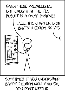
Think-pair-share: explain why Bill Gate’s reasoning is flawed in Figure 9.10 (thanks to Richard McElreath for tweeting this out!):

Figure 9.10: Tweet from Bill Gates that mixes up marginal and conditional probabilities.

9.9 Probability distributions in R

This section closely follows Jack Weiss’s lecture notes from his various classes. There are 4 basic probability functions associated with each probability distribution in R. These functions start with either - d, p, q, or r - and are then followed by a shortened name that identifies the distribution :

• d is for density and returns the value of f(y), i.e., the value of the probability density function (continuous distributions) or probability mass function (discrete distributions).

• p is for probability; returns a value of F(y), the cumulative distribution function.

• q is for quantile; returns a value from the inverse of F(y) and is also known as the quantile function.

• r is for random; generates a random value from the given distribution.

Let’s consider these 4 functions in the context of the Normal distribution with mean 0 and standard deviation 1. The functions are named dnorm, pnorm, qnorm, rnorm and are depicted in Figure 9.11.

Figure 9.11: Figure created using code written by Jack Weiss and made available in his course notes depicting the 4 basic probability functions for working with the Normal distribution in R.

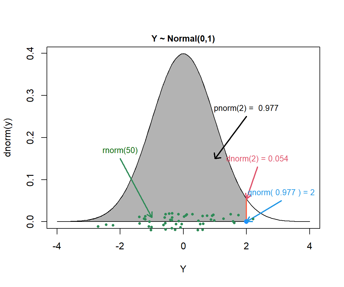
• dnorm(2)² or returns the value of the probability density function at $Y=2$, i.e., $f(2)$. Because the Normal distribution is continuous, this is not a probability; rather, we can integrate the probability density function over an interval to determine the probability that $Y$ falls in the interval. To visualize a probability density function or probability mass function, we can plot d* over a range of Y values.

• pnorm(2) returns the value of the cumulative distribution function, $F(2)=P(Y\le 2)=0.977$ for the Normal distribution. This probability is equal to the area under the Normal density curve to the left of $Y=2$ and is shaded gray in Figure 9.11.

• qnorm(0.977 returns the quantile function and determines the value of $Y$ such that $P(Y\le y)=0.977$.

• rnorm(50) generates 50 random values from a standard normal distribution, represented by the green points in Figure 9.11.

9.10 A sampling of discrete random variables

In the next few sections, we will consider several discrete and continuous probability distributions that are commonly used to model data or to test hypotheses in statistics.

9.10.1 Bernoulli distribution: $Y\sim$ Bernoulli($p$)

The Bernoulli distribution is used to model discrete random variables that can take on only two possible values, 1 or 0, with probabilities $p$ and $1-p$, respectively. The probability mass function of a Bernoulli distribution is given by:

$$f(y;p)=P(Y=y)=p^y(1-p{)}^{1-y}$$

Characteristics:

• Parameter: $p$, often referred to as the probability of ‘success’ = $P(Y=1)$, with $0\le p\le 1$
• Support (i.e., range of values that $Y$ can take on): $Y\in$ {0,1}
• $E[Y]=\sum yf(y;p)$ $=0(1-p)+1p=p$
• $Var[Y]=\sum (y-E[y]{)}^{2}f(y;p)$ $=(0-p{)}^2(1-p)+(1-p{)}^{2}p=p(1-p)$
• R does not contain functions specific to the Bernoulli distribution; rather, we have to work with functions for the Binomial distribution, which we will see next.
• JAGS and WinBugs: dbern

9.10.2 Binomial distribution $Y\sim$ Binomial$(n,p)$

A binomial random variable counts the the number of successes in a set of $n$ independent and identical Bernoulli trials, each with probability of success, $p$. IF

$$\begin{array}{r}{X}_i\sim Bernoulli(p)(i=1,2,\dots n)\\ Y=X_1+X_2+\dots X_n\end{array}$$

then, $Y\sim Binomial(n,p)$. The probability mass function for the Binomial distribution is given by:

$$P(Y=y)=(\genfrac{}{}{0ex}{}{n}{y})p^y(1-p{)}^{n-y}$$

The combinatoric term, $(\genfrac{}{}{0ex}{}{n}{y})$ (“n choose y”), arises from considering all possible trial sequences that give $y$ successes regardless of when those successes occur and is given by:

$$(\genfrac{}{}{0ex}{}{n}{y})=\frac{n!}{y!(n-y)!}\text{ with }n!=n(n-1)(n-2)\cdots (2)1$$

In our chronic wasting disease testing example (with $n$ = 2), we could end up with 1 positive test if either the first deer or the second deer tested positive and the other tested negative. This led us to calculate $P(Y=1)=p(1-p)+(1-p)p=(\genfrac{}{}{0ex}{}{2}{1})p^1(1-p{)}^1=2p(1-p)$.

Characteristics:

• Typically, the number of trials is assumed fixed and known, leaving a single parameter $p$ with $0\le p\le 1.$ In ecology, however, there are many instances where $n$ (usually written as $N$) is also an unknown parameter that we hope to estimate (e.g., population size in mark-recapture studies).
• Support: $Y\in [0,1,\dots n]$
• $E[Y]=np$
• $Var[Y=np(1-p)$
• R: dbinom, pbinom, qbinom, rbinom with arguments size = $n$ and prob = $p$
• JAGS: dbin(p, n)

Uses: a Bernoulli or binomial distribution is often used to model presence/absence and detection/non-detection data from wildlife surveys. It can also be used to model survival (Y/N), the number of eggs in a clutch that will hatch (or number of chicks that will fledge), etc.

Figure 9.12: Signed picture of Raymond Felton with a picture of Raymond Fieberg in the corner as a baby.

Example: Raymond Felton, a point guard on the University of North Carolina’s 2005 National Championship team, shot free throws at a 70% success rate during the 2004-2005 season. If we assume each of his free throw attempts can be modeled as independent trials, what is the probability that he would hit at least 4 out of 6 free throws in the 2005 Championship Game (he hit 5)?³

There are several ways to compute this probability in R:

1. Using $P(X\ge 4)=P(X=4)+P(X=5)+P(X=6)$ and the expression for the probability mass function:

choose(6,4)*(0.7)^4*(0.3)^2 + 
  choose(6,5)*(0.7)^5*(0.3) +
  0.7^6

[1] 0.74431

2. Using R’s built in probability mass function, dbinom:

sum(dbinom(4:6, size = 6, p = 0.70))

[1] 0.74431

3. Using R’s built in cumulative distribution function, pbinom, and recognizing that $P(Y\ge 4)=1-P(Y\le 3)$.

1- pbinom(3, size = 6, p = 0.7)

NA [1] 0.74431

4. We can also use pbinom with the argument lower.tail = FALSE, which will give us $P(Y>y)=P(Y\ge y+1)$ for discrete random variables.

pbinom(3, size = 6, p = 0.7, lower.tail= FALSE)

[1] 0.74431

9.10.3 Geometric distribution

The Geometric distribution arises from considering the number of failures until you get your first success in a set of Bernoulli random trials. To derive the probability mass function for the Geometric distribution, note that we have to have $y$ failures (each with probability $1-p$) followed by a single success with probability $p$:

$$f(y;p)=P(Y=y)=(1-p{)}^{y}p$$

• Parameter: $p$ (probability of success), with $0\le p\le 1$
• Support: $Y\in [0,1,2,\dots ,\mathrm{\infty }]$
• $E[Y]=\frac{1}{p}-1$
• $Var[Y]=\frac{(1-p)}{p^2}$
• R: *geom with parameter prob = $p$
• JAGS: dnegbin(p, 1)

Other notes:

Sometimes the Geometric distribution is defined as the number of trials until the first success. In this case, the probability mass function is defined as:

$$f(y)=P(Y=y)=(1-p{)}^{(y-1)}p$$

with support: $Y\in [1,2,\dots ,\mathrm{\infty }]$ and $E[Y]=\frac{1}{p}$, $Var[Y]=\frac{(1-p)}{p^2}$

9.10.4 Multinomial distribution $Y\sim$ Multinomial$(n,p_1,p_2,\dots ,p_k)$

The multinomial distribution is a generalization of the binomial distribution, allowing for $k$ possible outcomes with probabilities ($p_1,p_2,\dots ,p_k$; $p_k=1-\sum _{i-1}^{k-1}{p}_i$)⁴. Let $n$ be the number of independent trials, $Y=(Y_1,Y_2,\dots ,Y_k)$ be a multivariate random variable recording the number of events in each category, and $(n_1,n_2,\dots ,n_k)$ give the observed number of events in each category, then the probability mass function is defined as:

$P((Y_1,Y_2,\dots ,Y_k)=(n_1,n_2,\dots ,n_k))=\frac{n!}{n_1!n_2!\cdots n_k!}{p}_1^{n_1}{p}_2^{n_2}\cdots p_k^{n_k}$

Characteristics:

• Parameters: $p_1,p_2,\dots ,p_k$ with $0\le p_i\le 1$ for all $i$. As with the binomial distribution, $n$ can also be viewed as an unknown parameter in various mark-recapture and wildlife abundance estimation frameworks (e.g., Otis et al. 1978; Pollock et al. 1990).
• R: dmultinom, pmultinom, qmultinom, rmultinom with parameters size = $n$ and prob = $p$.
• JAGS: dmulti(p,n)

Uses:

The multinomial distribution is often appropriate for modeling a categorical response variable with more than 2 unordered categories. The multinomial distribution frequently arises when modeling capture histories in mark-recapture studies (e.g., Otis et al. 1978; Pollock et al. 1990).

9.10.5 Poisson distribution: $Y\sim Poisson(\lambda )$

The Poisson distribution is often used to model counts of events randomly distributed in space or time, occurring at a rate, $\lambda$. Let $Y_t$ = the number of events occurring in a time interval of length $t$. The probability mass function in this case is given by:

$$P(Y_t=y)=\frac{\exp (-\lambda t)(\lambda t{)}^y}{y!}$$

Similarly, let $Y_A$ the number of events occurring in a spatial unit of area $A$. Then,

$$P(Y_A=y)=\frac{\exp (-\lambda A)(\lambda A{)}^y}{y!}$$

Oftentimes, observations are recorded over constant time intervals or spatial units all of the same size. In this case, the probability mass function would be defined simply as:

$$P(Y=y)=\frac{\exp (-\lambda )(\lambda {)}^y}{y!}$$

Characteristics:

• Parameter: $\lambda \ge 0$
• Support: $Y\in [0,1,2,\dots ,\mathrm{\infty }]$
• $E[Y]=Var[Y]=\lambda$
• R: dpois, ppois, qpois, and rpois with parameter lambda.
• JAGS: dpois(lambda)

Uses: the Poisson distribution is often used as a null model in spatial statistics. Although it can be used as a general model for count data, most ecological data are “overdispersed”, meaning that $Var[Y]\gg E[Y]$, and thus, the Poisson distribution often does not fit well.

Example: suppose a flower bed receives, on average, 10 visits by Monarchs a day in mid-August. Further, assume the number of daily visits closely follows a Poisson distribution. What is the probability of seeing 15 monarchs on a random visit to the garden?

dpois(15, lambda=10)

[1] 0.03471807

10^15*exp(-10)/(factorial(15)) 

[1] 0.03471807

9.10.6 Negative Binomial

9.10.6.1 Classic parameterization $Y\sim$ NegBin($p,r$)

There are 2 different parameterizations of the Negative Binomial distribution, which we will refer to as the “classic” and “ecological” parameterizations. Consider again a set of independent Bernoulli trials. Let $Y$ = number of failures before the $r^{th}$ success. To derive the probability mass function for the classic parameterization of the Negative Binomial distribution, consider:

• We will have a total of $n=y+r$ trials
• The last trial will be a success (with probability $p$)
• The preceding $y+r-1$ trials will have had $y$ failures and can be described by the binomial probability mass function with $n=y+r-1$ and $p$.

$P(Y=y)=(\genfrac{}{}{0ex}{}{y+r-1}{y})p^{r-1}(1-p{)}^{y}p=(\genfrac{}{}{0ex}{}{y+r-1}{y})p^r(1-p{)}^y$

Characteristics:

• Parameters: r must be integer valued and > 0, $0\le p\le 1$
• Support: $Y\in [0,1,2,\dots ,\mathrm{\infty }]$
• $E[Y]=\frac{r(1-p)}{p}$
• $Var[Y]=\frac{r(1-p)}{p^2}$
• In R: *nbinom, with parameters (prob = p, size = $n$)

9.10.6.2 Ecological parameterization $Y\sim$ NegBin($\mu ,\theta$)

To derive the ecological parameterization of the Negative Binomial distribution, we express $p$ in terms of the mean, $\mu$ and $r$:

$$\begin{array}{r}\mu =\frac{r(1-p)}{p}\Rightarrow p=\frac{r}{\mu +r}and\\ 1-p=\frac{\mu }{\mu +r}\end{array}$$

Plugging these values in to $f(y)$ and changing $r$ to $\theta$, we get:

$P(Y=y)=(\genfrac{}{}{0ex}{}{y+\theta -1}{y}){\left(\frac{\theta }{\mu +\theta }\right)}^{\theta }{\left(\frac{\mu }{\mu +\theta }\right)}^y$

Then, let $\theta$ = dispersion parameter take on any positive number (not just integers as in the original parameterization).

Characteristics:

• Parameters: $\mu \ge 0$, $\theta >0$
• $E[Y]=\mu$
• $Var[Y]=\mu +\frac{{\mu }^2}{\theta }$
• in R: *nbinom, with parameters mu = $\mu$, size = $\theta$
• JAGS: dnegbin with parameters ($p$, $\theta$)

Uses: the Negative Binomial model is often used to model overdispersed count data where the variance is greater than the mean. Note that as $\theta \to \mathrm{\infty }$, the Negative Binomial distribution approaches the Poisson. In my experience, the Negative Binomial model almost always provides a better fit to ecological count data than the Poisson.

Other notes: if $Y_i\sim$ Poisson(${\lambda }_i$), with ${\lambda }_i\sim$ Gamma($\alpha ,\beta$), then $Y_i$ will have a negative binomial distribution.

9.11 A sampling of continuous probability distributions

9.11.1 Normal Distribution $Y\sim N(\mu ,{\sigma }^2)$

The probability density function for the normal distribution is given by:

$$f(y;\mu ,\sigma )=\frac{1}{\sqrt{2\pi }\sigma }\exp (-\frac{(y-\mu {)}^2}{2{\sigma }^2})$$

Characteristics:

• Parameters: $\mu \in (-\mathrm{\infty },\mathrm{\infty })$ and $\sigma >0$
• $E[Y]=\mu$
• $Var[Y]={\sigma }^2$.
• Support: $Y\in (-\mathrm{\infty },\mathrm{\infty })$.
• R: dnorm, pnorm, qnorm, rnorm; these functions have arguments for the mean and standard deviation, sd, of the Normal distribution
• JAGS: also has a dnorm function, but it is specified in terms of the precision, $\tau =1/{\sigma }^2$, rather than standard deviation

Uses: the Normal distribution forms the backbone of linear regression. The Central Limit Theorem tells us that as $n$ gets large, $\overline{y}$ and $\sum y$ become Normally distributed. Thus, the Normal distribution serves as a useful model for response variables influenced by a large number of factors that act in an additive way. The Normal distribution is also often used to define prior distributions in Bayesian analysis.

Other notes: one of the really unique characteristics of the Normal distribution is that the mean and variance are independent (knowing the mean tells us nothing about the variance and vice versa). By contrast, most other probability distributions have parameters that influence both the mean and variance (e.g., the mean and variance of a binomial random variable are $np$ and $np(1-p)$). Thus, although it is possible to define linear regression models in terms of a model for the mean + and independent error term, this will not be the case for other probability distributions. The error (or variability about the mean) will usually depend on the mean itself! We will revisit this point when we learn how to write expressions for regression models formulated using statistical distributions other than the Normal distribution.

Special cases: setting $\mu =0$ and $\sigma =1$ gives us the standard normal distribution $Y\sim N(0,1)$.

9.11.2 log-normal Distribution: $Y\sim$ Lognormal$(\mu ,\sigma )$

$Y$ has a log-normal distribution of if $\log (Y)\sim N(\mu ,{\sigma }^2)$. The probability density function for the log-normal distribution is given by:

$$f(y;\mu ,\sigma )=\frac{1}{y\sqrt{2\pi }\sigma }\exp (-\frac{(log(y)-\mu {)}^2}{2{\sigma }^2})$$

Characteristics:

• Parameters: $\mu$ and $\sigma >0$ are the mean and variance of log($Y$) not $Y$
• Support: $Y\in (0,\mathrm{\infty })$
• $E[Y]=\exp (\mu +1/2{\sigma }^2)$
• $Var(Y)=\exp (2\mu +{\sigma }^2)(\exp ({\sigma }^2)-1)$
• $Var(Y)=kE[Y{]}^2$
• R: dlnorm, plnorm, qlnorm, rlnorm with parameters meanlog and sdlog
• JAGS: dlnorm(meanlog, 1/varlog)

Uses: whereas the Normal distribution provides a reasonable model for response variables formed by adding many different factors together, the lognormal distribution serves as a useful model for response variables formed by multiplying many independent factors together. This follows again from the Central Limit Theorem since $log(Y_1{Y}_2\cdots Y_n)=log(Y_1)+log(Y_2)+\dots log(Y_n)$, and hence, as $n$ gets large, $\sum log(y)/n$) will converge in distribution to a Normal. The lognormal distribution arises naturally in the case of stochastic population models formulated in discrete time: $N_t={\lambda }_t{N}_{t-1}$, where $N_t$ is the population size at time $t$ (Morris et al. 1999).

9.11.3 Continuous Uniform distribution: $Y\sim U(a,b)$

If observations are equally likely within an interval $(a,b)$:

$$f(y;a,b)=\frac{1}{b-a}$$

Characteristics:

• Parameters: $(a,b)$ which together defined the support of $Y\in (a,b)$
• $E[Y]=(a+b)/2$
• $Var[Y]=\sqrt{(b-a{)}^2/12}$
• R: *unif with min = a, max = b
• JAGS: dunif(lower, upper)

Uses: the uniform distribution is often used as a model of ignorance for prior distributions. Also, p-values across replicated experiments in which the null hypothesis is true should follow a uniform distribution.

9.11.4 Beta Distribution: $Y\sim$ Beta($\alpha ,\beta$)

The Beta distribution is unique in that it has support only on the (0,1) interval, which makes it useful for modeling probabilities (or as a prior distribution for $p$ when modeling binary data). The probability density function for the Beta distribution is given by:

$$f(y;\alpha ,\beta )=\frac{\mathrm{\Gamma }(\alpha +\beta )}{\mathrm{\Gamma }(\alpha )\mathrm{\Gamma }(\beta )}{y}^{\alpha -1}(1-y{)}^{\beta -1}$$

This is the first time we have seen the gamma function ($\mathrm{\Gamma }$), which is defined as:

$$\mathrm{\Gamma }(x)={\int }_0^{\mathrm{\infty }}{t}^{x-1}{e}^{-t}dt$$

The gamma function generalizes factorials ($x$!) to non-integer values; for any integer, $n$, $\mathrm{\Gamma }(n)=(n-1)!$ In R, the gamma function can be executed using gamma(n), e.g., gamma(4) = 3! = $3\ast 2\ast 1$ = 6:

gamma(4)

[1] 6

Characteristics:

• Parameters: $\alpha >0$ and $\beta >0$
  
• Support: $Y\in (0,1)$
• $E[Y]=\frac{\alpha }{\alpha +\beta }$
• $Var[Y]=\frac{\alpha }{(\alpha +\beta {)}^2(\alpha +\beta +1)}$
• R: *beta with shape1 = $\alpha$ and shape2 = $\beta$
• JAGS: dbeta

Uses: the Beta distribution is sometimes used to model probabilities or proportions (in cases where the number of trials is not known). It is also frequently used as a prior distribution for $p$ when modeling binary data.

Special cases: when $\alpha =\beta =1$, we get a continuous uniform(0,1) distribution.

9.11.5 Exponential: $Y\sim$ Exp($\lambda$)

If we have a random (Poisson) event process with rate parameter, $\lambda$, then the wait time between events follows an exponential distribution. The probability density function for the exponential distribution is given by:

$$f(y;\lambda )=\lambda \exp (-\lambda y)$$

Characteristics:

• Parameter: $\lambda >0$
• Support: $Y\in (0,\mathrm{\infty })$
• $E[Y]=\frac{1}{\lambda }$
• $Var[Y]=\frac{1}{{\lambda }^2}$
• R: *exp with rate = $\lambda$
• JAGS: dexp

Uses: often used to model right-skewed distributions, particularly in time-to-event models.

9.11.6 Gamma Distribution: $Y\sim$ Gamma($\alpha ,\beta$)

If we have a random (Poisson) event process with rate parameter, $\lambda$, then the waiting time before $\alpha$ events occur follows a Gamma distribution. The probability density function for the Gamma distribution is given by:

$$f(y;\alpha ,\beta )=\frac{1}{\mathrm{\Gamma }(\alpha )}{y}^{\alpha -1}{\beta }^{\alpha }\exp (-\beta y)$$

• Parameters: $\alpha >0$ and $\beta >0$
• Support: $Y\in (0,\mathrm{\infty })$
• $E[Y]=\frac{\alpha }{\beta }$
• $Var[Y]=\frac{\alpha }{{\beta }^2}$
• R: *gamma with shape = $\alpha$ and rate = $\beta$, or shape = $\alpha$ and scale = $1/\beta$
• JAGS: dgamma(alpha, beta)

Uses: the Gamma distribution can be used to model non-negative continuous random variables. In movement ecology, the Gamma distribution is often used to model step-lengths connecting consecutive telemetry locations $\mathrm{\Delta }t$ units apart (e.g., Signer, Fieberg, and Avgar 2019; Fieberg et al. 2021).

Special cases: when $\alpha =1$, we get an exponential distribution with rate parameter $\beta$. A Gamma distribution with $\alpha =k/2$ and $\beta =1/2$ is a chi-squared distribution with $k$ degrees of freedom, ${\chi }_k^2$.

9.12 Some probability distributions used for hypotheses testing

9.12.1 ${\chi }^2$ distribution: $Y\sim {\chi }_{df=k}^2$

The ${\chi }^2$ distribution is often encountered in introductory statistics classes where it is used for goodness-of-fit testing for a single categorical variable and for constructing tests of association between two categorical variables (Agresti 2018). We will also encounter the ${\chi }^2$ distribution when comparing nested models using likelihood ratio tests. Lastly, the ${\chi }^2$ distribution is used to construct confidence intervals for the variance of Normally distributed random variables since $(n-1)s^2/{\sigma }^2$ will follow a ${\chi }^2$ distribution with $n-1$ degrees of freedom in this case.

The probability density function for the ${\chi }^2$ distribution with $k$ degrees of freedom is given by:

$$f(y;k)=\frac{y^{k/2-1}\exp (-y/2)}{2^{k/2}\mathrm{\Gamma }(k/2)}$$

Characteristics:

• Parameter: $k>0$
• Support: $Y\in (0,\mathrm{\infty })$
• $E[Y]=k$
• $Var[Y]=2k$
• R: *chisq with df = $k$
• JAGS: dchisqr(k)

9.12.2 Student’s t distribution $Y\sim t_{df=k}$

We encountered the t-distribution in Chapter 1, which we used to test hypotheses involving individual coefficients in our regression models. The probability density function for the student t distribution with $k$ degrees of freedom is given by:

$$f(y;k)=\frac{\mathrm{\Gamma }(\frac{k+1}{2})}{\mathrm{\Gamma }(\frac{k}{2})\sqrt{k\pi }}(1+\frac{y^2}{k}{)}^{-(\frac{k+1}{2})}$$

Characteristics:

• Parameter: $k>0$; can also include a non-centrality parameter (e.g., used when calculating power of hypothesis tests)
• Support: $Y\in (-\mathrm{\infty },\mathrm{\infty })$
• $E[Y]=0$
• $Var[Y]=k/(k-2)$ for $k>2$
• R: *t with df = $k$, ncp = non-centrality parameter
• JAGS: dt(mu, tau, k), with tau=1, then mu is equal to the non-centrality parameter in R and k is the degrees of freedom

9.12.3 F distribution, $Y\sim F_{d{f}_1=k_1,d{f}_2=k_2}$

We saw the F-distribution when testing whether multiple coefficients associated with a categorical predictor were simultaneously 0 in Section 3.10. The probability density function for the F-distribution with $k_1$ and $k_2$ degrees of freedom is given by:

$$f(y;k_1,k_2)=\frac{\mathrm{\Gamma }((k_1+k_2)/2)(k_1/k_2{)}^{k_1/2}{y}^{k_1/2-1}}{\mathrm{\Gamma }(k_1/2)\mathrm{\Gamma }(k_2/2)[(k_1/k_2)y+1{]}^{(k_1+k_2)/2}}$$

Characteristics:

• Parameter: $k_1,k_2>0$; can also include a non-centrality parameter (e.g., used when calculating power of hypothesis tests)
• Support: $Y\in (0,\mathrm{\infty })$
• $E[Y]=\frac{k_2}{k_2-2},k_2>0$
• $Var[Y]=2{\left(\frac{k_2}{k_2-2}\right)}^2\frac{(k_1+k_2-2)}{k_1(k_2-4)},k_2>4$
• R: *f with df1 = $k_1$, df2 = $k_2$, ncp = non-centrality parameter
• JAGS: df

9.13 Choosing an appropriate distribution

How do we choose an appropriate distribution for our data? This may seem like a difficult task after having just been introduced to so many new statistical distributions. In reality, you can usually whittle down your choices to a few different distributions by just considering the range of observations and the support of available distributions. For example:

• If your data are continuous and can take on any value between $(-\mathrm{\infty },\mathrm{\infty })$, or if the range is small relative to the mean, then the Normal distribution is usually a good default.
• If your data are continuous, non-negative, and right-skewed, then a log-normal or gamma distribution is likely appropriate; if your data also contain zeros, then you may need to consider a mixture distribution (see Chapter 17).
• If you are modeling binary data that can take on only 1 of 2 values (e.g., alive/dead, present/absent, infected/not-infected), then a Bernoulli distribution is appropriate.
• If you have a count associated with a fixed number of “trials” (e.g., $Y$ out of $n$ individuals are alive, infected, etc.), then a Binomial distribution is a good default.
• If you have counts associated with temporal or spatial units, then you might consider the Poisson or Negative Binomial distributions (or zero-inflated versions that we will see later).
• If you are modeling time-to-event data (e.g., as when conducting a survival analysis), then you might consider the exponential distribution, gamma distribution, or a generalization of the gamma called the Weibull distribution.
• If you have circular data (e.g., your response is an angle or a time between 0 and 24 hours or 0 and 365 days), then you would likely want to consider specific distributions that allow for periodicities (e.g., 0 is the same as 2$\pi$; 0:00 is equivalent to 24:00 hours). Examples include the von Mises distribution or various “wrapped distributions” like the wrapped Normal distribution (Pewsey, Neuhäuser, and Ruxton 2013).

9.14 Summary of statistical distributions

You may find it useful to visualize different statistical distributions. This site is great! You can choose from many different statistical distributions and vary their parameters to see how it changes the probability (mass or density) function and the cumulative density function! Thanks to Jeremiah Shrovnal for pointing me to it!

Table 9.2 briefly details most of the random variables discussed in this chapter and was modified from this site.

Table 9.2: Review of mentioned random variables.

Distribution Name	pmf / pdf	Parameters	Possible Y Values	Description
Bernouli	$p^Y(1-p{)}^{1-Y}$	$p$	$0,1$	Success or failure
Binomial	$(\genfrac{}{}{0ex}{}{n}{y})p^y(1-p{)}^{n-y}$	$p,n$	$0,1,\dots ,n$	Number of successes after $n$ trials
Geometric	$(1-p{)}^{y}p$	$p$	$0,1,\dots ,\mathrm{\infty }$	Number of failures until the first success
Multinomial	$\frac{n!}{n_1!n_2!\cdots n_k!}{p}_1^{n_1}{p}_2^{n_2}\cdots p_k^{n_k}$	$p_i,i=1,2,\dots k$	$0,1,\dots ,n$ for each $Y_i$	Number of successes associated with each of $k$ categories
Poisson	$e^{-\lambda }{\lambda }^y/y!$	$\lambda$	$0,1,\dots ,\mathrm{\infty }$	Number of events in a fixed time interval or spatial unit
Negative Binomial (classic)	$(\genfrac{}{}{0ex}{}{y+r-1}{y})(p{)}^r(1-p{)}^y$	$r,p$	$0,1,\dots ,\mathrm{\infty }$	Number of failures before $r$ successes
Negative Binomial (ecological)	$(\genfrac{}{}{0ex}{}{y+\theta -1}{y}){\left(\frac{\theta }{\mu +\theta }\right)}^{\theta }{\left(\frac{\mu }{\mu +\theta }\right)}^y$	$\mu ,\theta$	$0,1,\dots ,\mathrm{\infty }$	A model for overdispersed counts
Normal	${\displaystyle \frac{e^{-(y-\mu {)}^2/(2{\sigma }^2)}}{\sqrt{2\pi {\sigma }^2}}}$	$\mu ,\sigma$	$(-\mathrm{\infty },\mathrm{\infty })$	Model for when a large number of factors act in an additive way
log-Normal	${\displaystyle \frac{e^{-(log(y)-\mu {)}^2/(2{\sigma }^2)}}{y\sqrt{2\pi }\sigma }}$	$\mu ,\sigma$	$(0,\mathrm{\infty })$	Model for when a large number of factors act in an multiplicative way
Uniform	$\frac{1}{b-a}$	$a,b$	$[a,b]$	Useful for specifying vague priors
Beta	$\frac{\mathrm{\Gamma }(\alpha +\beta )}{\mathrm{\Gamma }(\alpha )\mathrm{\Gamma }(\beta )}{y}^{\alpha -1}(1-y{)}^{\beta -1}$	$\alpha ,\beta$	$(0,1)$	Useful for modeling probabilities
Exponential	$\lambda e^{-\lambda y}$	$\lambda$	$(0,\mathrm{\infty })$	Wait time for one event in a Poisson process
Gamma	${\displaystyle \frac{{\lambda }^r}{\mathrm{\Gamma }(r)}{y}^{r-1}{e}^{-\lambda y}}$	$\alpha ,\beta$	$(0,\mathrm{\infty })$	Wait time for $r$ events in a Poisson process
${\chi }^2$	$\frac{y^{k/2-1}{e}^{(-y/2)}}{2^{k/2}\mathrm{\Gamma }(k/2)}$	$k$	$(0,\mathrm{\infty })$	Distribution for goodness-of-fit tests, likelihood ratio test
Students t	$\frac{\mathrm{\Gamma }(\frac{k+1}{2})}{\mathrm{\Gamma }(\frac{k}{2})\sqrt{k\pi }}(1+\frac{y^2}{k}{)}^{-(\frac{k+1}{2})}$	$k$	$(-\mathrm{\infty },\mathrm{\infty })$	Distribution for testing hypotheses involving means, regression coefficients
F	$\frac{\mathrm{\Gamma }((k_1+k_2)/2)(k_1/k_2{)}^{k_1/2}{y}^{k_1/2-1}}{\mathrm{\Gamma }(k_1/2)\mathrm{\Gamma }(k_2/2)[(k_1/k_2)y+1{]}^{(k_1+k_2)/2}}$	$k_1,k_2$	$(0,\mathrm{\infty })$	Distribution for testing hypotheses involving regression coefficients

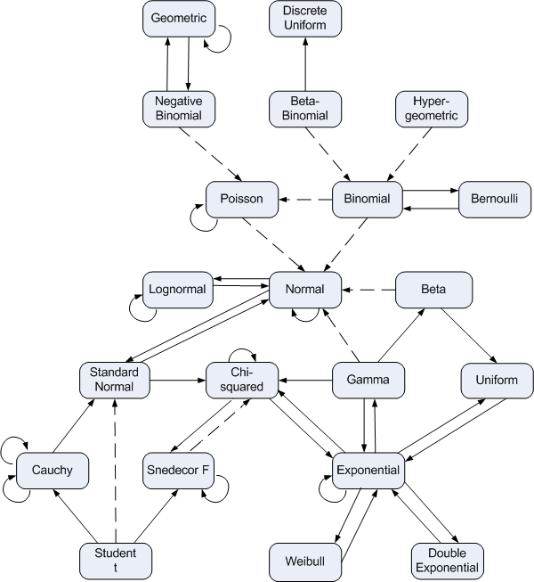
In a few places, we have highlighted connections among different statistical distributions, but there are many other connections that we did not mention (e.g., see Figure 9.13).

Figure 9.13: Relationships among some of univariate probability distributions. Figure from https://www.johndcook.com/blog/distribution_chart/.

9.15 References

Agresti, Alan. 2018. An Introduction to Categorical Data Analysis. John Wiley & Sons.

Bramwell, Ros, Helen West, and Peter Salmon. 2006. “Health Professionals’ and Service Users’ Interpretation of Screening Test Results: Experimental Study.” Bmj 333 (7562): 284.

Fieberg, John, Johannes Signer, Brian Smith, and Tal Avgar. 2021. “A ‘How to’ Guide for Interpreting Parameters in Habitat-Selection Analyses.” Journal of Animal Ecology 90 (5): 1027–43.

Forstmeier, Wolfgang, Eric-Jan Wagenmakers, and Timothy H Parker. 2017. “Detecting and Avoiding Likely False-Positive Findings–a Practical Guide.” Biological Reviews 92 (4): 1941–68.

Herbranson, Walter T, and Julia Schroeder. 2010. “Are Birds Smarter Than Mathematicians? Pigeons (Columba Livia) Perform Optimally on a Version of the Monty Hall Dilemma.” Journal of Comparative Psychology 124 (1): 1.

Ioannidis, John PA. 2005. “Why Most Published Research Findings Are False.” PLoS Medicine 2 (8): e124.

MacKenzie, Darryl I, James D Nichols, J Andrew Royle, Kenneth H Pollock, Larissa Bailey, and James E Hines. 2017. Occupancy Estimation and Modeling: Inferring Patterns and Dynamics of Species Occurrence. Elsevier.

Morris, William, Daniel Doak, Martha Groom, Peter Kareiva, John Fieberg, Leah Gerber, Peter Murphy, and Diane Thomson. 1999. “A Practical Handbook for Population Viability Analysis.” The Nature Conservancy.

Otis, David L, Kenneth P Burnham, Gary C White, and David R Anderson. 1978. “Statistical Inference from Capture Data on Closed Animal Populations.” Wildlife Monographs, no. 62: 3–135.

Pewsey, Arthur, Markus Neuhäuser, and Graeme D Ruxton. 2013. Circular Statistics in r. Oxford University Press.

Pollock, Kenneth H, James D Nichols, Cavell Brownie, and James E Hines. 1990. “Statistical Inference for Capture-Recapture Experiments.” Wildlife Monographs, 3–97.

Ponisio, Lauren C, Perry de Valpine, Nicholas Michaud, and Daniel Turek. 2020. “One Size Does Not Fit All: Customizing MCMC Methods for Hierarchical Models Using NIMBLE.” Ecology and Evolution 10 (5): 2385–2416.

Roback, Paul, and Julie Legler. 2021. Beyond Multiple Linear Regression: Applied Generalized Linear Models and Multilevel Models in r. Chapman; Hall/CRC.

Signer, Johannes, John Fieberg, and Tal Avgar. 2019. “Animal Movement Tools (Amt): R Package for Managing Tracking Data and Conducting Habitat Selection Analyses.” Ecology and Evolution 9 (2): 880–90.

Weber, Patrick, Karin Binder, and Stefan Krauss. 2018. “Why Can Only 24% Solve Bayesian Reasoning Problems in Natural Frequencies: Frequency Phobia in Spite of Probability Blindness.” Frontiers in Psychology 9: 1833.

Yackulic, Charles B, Michael Dodrill, Maria Dzul, Jamie S Sanderlin, and Janice A Reid. 2020. “A Need for Speed in Bayesian Population Models: A Practical Guide to Marginalizing and Recovering Discrete Latent States.” Ecological Applications 30 (5): e02112.

---

1. A countably infinite set of values can be put in a 1-1 correspondence with the set of non-negative integers.

2. Note, we have ignored the other arguments to this function, which include mean and sd, allowing them to take on their default values of 0 and 1.

3. I became a huge University of North Carolina basketball fan after going to graduate school in Chapel Hill and attending nearly every home basketball game for 6 years. My son is named after Raymond Felton, the point guard from the 2005 National Championship team and my youngest daughter is named Carolina Anne. I had plane tickets to join friends of mine in Chapel Hill to watch the 2005 Championship game, but ultimately decided not to go. My oldest daughter, Zoe, was only 2 weeks old. I had also witnessed 4 final four losses during my time in North Carolina. Ultimately, I decided to watch the game with my wife and daughter at home.

4. Once we know $k-1$ of the $p_i$’s, we can determine the last one since they must sum to 1.