This book is in Open Review. I want your feedback to make the book better for you and other readers. To add your annotation, select some text and then click the on the pop-up menu. To see the annotations of others, click the in the upper right hand corner of the page

10  Maximum likelihood

Learning objectives

1. Understand how to use maximum likelihood to estimate parameters in statistical models.

2. Understand how to create large-sample confidence intervals for parameters estimated using maximum likelihood.

3. Be able to construct large-sample confidence intervals for functions of parameters using the delta method.

4. Be able to conduct likelihood ratio tests for nested models and understand that profile-likelihood intervals can be formed by inverting the likelihood ratio test.

Credit: much of this material in this section was originally developed by Jack Weiss and presented online as part of his Statistical Ecology courses at the University of North Carolina.

10.1 R packages

We begin by loading a few packages upfront:

library(kableExtra) # for creating tables 
options(kableExtra.html.bsTable = T)
library(dplyr) # for data wrangling
library(ggplot2) # for plotting
library(patchwork) # for creating multi-panel plots

In addition, we will use data and functions from the following packages:

• Data4Ecologists for beargrowth and slugs data sets
• emdbook (B. Bolker 2023) for the deltavar function used to calculate standard errors via the delta method.

10.2 Parameter estimation

In the previous section, we learned about a number of statistical distributions, described by a small set of parameters. We might now ask:

• How do we determine appropriate values of the parameters?
• How do we incorporate the effects of covariates on these parameters and thus, the distributions of our data?
• How do we calculate confidence intervals or conduct hypotheses tests associated with these parameters?

Although there are alternative approaches (e.g., least squares, methods of moments), we will focus on two primary methods for estimating parameters:

• Maximum likelihood estimators
• Bayesian inference

Most statistical software packages use maximum likelihood to estimate parameters, including for example, the glm function in R for fitting logistic and Poisson regression models that will be the subject of later Sections of this book. Although users do not necessarily need to know the details of how maximum likelihood works in order to apply these methods, this knowledge will be helpful for understanding the inferential framework associated with commonly used statistical models fit in a frequentist framework (e.g., SEs and confidence intervals usually rely on an assumption that the sampling distribution is Normal, which will be reasonable for parameters estimated using maximum likelihood as long as our sample sizes are large or the data are Normally distributed). Typically, numerical analysis methods are needed to estimate parameters using maximum likelihood. You will be introduced to these methods, which may seem like a bit of a diversion. Yet, this knowledge will allow you to formulate and fit custom models that may otherwise not be available in current software. Lastly, likelihoods are also a key component of Bayesian inferential techniques. Thus, this section will help to prepare you for your journey into Bayesian inference.

To help motivate this section, consider the weight-at-age relationship for female black bears monitored in Minnesota depicted in Figure 10.1, constructed using the code below.

library(Data4Ecologists)
theme_set(theme_bw())
data(beargrowth)
beargrowth <- beargrowth %>% filter(sex=="Female")
ggplot(beargrowth, aes(age, wtkg)) + 
  geom_point() + geom_smooth() + ylab("Weight (kg)") + xlab("Age (years)")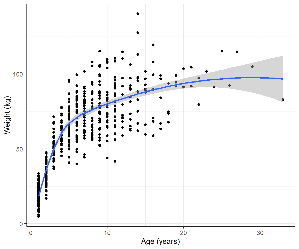 

Figure 10.1: Weight versus age depicted for black bears monitored in Minnesota.

We see that the pattern is non-linear and also that the variance of the observations increases with the age of the bears. We could try to model these data using polynomials or splines (see Chapter 4) combined with a variance model from Chapter 5. However, there are also many non-linear functions that have “built-in” asymptotes, and these are frequently used to model growth rates. Here, we will consider the von Bertalanffy growth function (Beverton and Holt 2012):

$$\begin{array}{}\text{(10.1)}& E[Y_i]=L_{\mathrm{\infty }}(1-e^{-K(Ag{e}_i-t_0)})\end{array}$$

An advantage of using a growth model like the von Bertalanffy growth curve versus a phenomenological model (e.g., using polynomials or splines) is that the model’s parameters often have useful biological interpretations. For example, $L_{\mathrm{\infty }}$ represents the asymptotic weight of individuals in the population.

Although there are R packages (e.g., FSA; Ogle et al. 2021) that allow one to fit the von Bertalanffy growth curve to data, by writing our own code and using built-in optimizers, we will be able to tailor our model to specific features of our data (e.g., we can relax the assumption that the variance about the mean growth curve is constant). We could relax the constant variance assumption using a GLS-style model or by using an alternative probability distribution (e.g., log-normal) that allows for non-constant variance. To accomplish this goal, we will need to be able to write some of our own code and also use built-in optimizers in R. Keep this example in mind when we go over numerical methods for estimating parameters using maximum likelihood.

10.3 Introductory example: Estimating slug densities

Crawley (2012) describe a simple data set consisting of counts of the number of slugs found beneath 40 tiles in each of two permanent grasslands. The data are contained within the Data4Ecologists library.

library(Data4Ecologists)
data(slugs)
str(slugs)

'data.frame':   80 obs. of  2 variables:
 $ slugs: int  3 0 0 0 0 1 0 3 0 0 ...
 $ field: chr  "Nursery" "Nursery" "Nursery" "Nursery" ...

Let’s begin by looking at the distribution of slug counts under the tiles in these two fields (Figure 10.2).

ggplot(slugs, aes(slugs, fill=field))+
  geom_bar(position=position_dodge())+
  theme(text = element_text(size=20))+
   scale_fill_manual(values=c("red", "blue"))+
   scale_x_continuous(breaks=seq(0,11,1))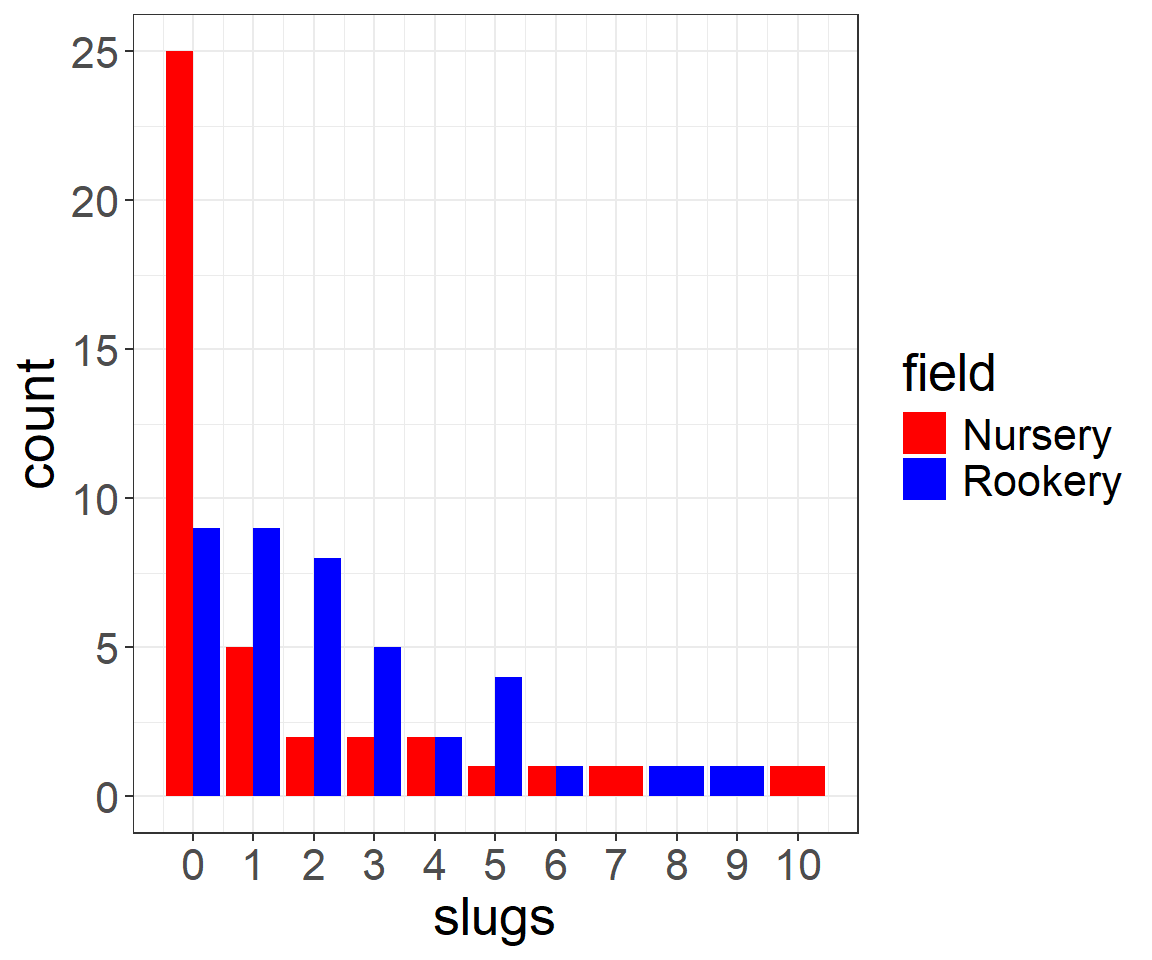

Figure 10.2: Distribution of slug counts under tiles placed in two fields.

We see that there are more slugs, on average, under the tiles located at the Rookery site than the Nursery site. Also note that the data take on only integer values $(0,1,\dots ,10)$ and that the distribution of slug counts is highly right skewed; this shape is typical of many count data sets. Thus, the data are not likely to be well described by a Normal distribution.

What if we wanted to conduct a formal hypothesis test to see whether the mean number of slugs per tile differed between the two sites? I.e., what if we wanted to test the Null Hypothesis, $H_0:{\mu }_{rookery}={\mu }_{nursery}$ versus the alternative hypothesis $H_A:{\mu }_{rookery}\ne {\mu }_{nursery}$?¹

We could consider using a two-sample t-test for a difference in means. In this case, what would we have to assume? At a minimum, we would need to assume that the observations are:

1. Independent
2. Normally distributed or that the sample size is “large enough” for the Central Limit Theorem (CLT) to apply

A common guideline is that $n\ge 30$ for the CLT to apply, with larger sample sizes needed when the population distributions are heavily skewed. Thus, we may be OK in this case due to having 40 observations in both fields. Nonetheless, we might consider whether there are more appropriate statistical distributions that we could use (instead of a Normal distribution) to describe the data from both fields. Given that we have count data, we might consider a Poisson or Negative Binomial distribution since these distributions also only take on integer values.

Let’s begin by assuming the counts at each site follow a Poisson distribution. We could then represent our null and alternative hypotheses using the models, below:

Null model:

$Y_i\sim Poisson({\lambda }_0)$ ($i=1,2,\dots ,80$)

Alternative model:

$Y_{ij}\sim Poisson({\lambda }_j)$ where $i=1,2,\dots ,40$ and $j=1,2$ for the Nursery and Rookery site, respectively.

OK, great - but, how do we estimate ${\lambda }_0$ and (${\lambda }_1,{\lambda }_2$)? And, how can we compare the two models to determine whether there is evidence to suggest the $\lambda$’s differ at the two sites?

10.4 Probability to the likelihood

To estimate parameters using Maximum Likelihood, we begin by writing down a probability statement reflecting an assumed data-generating model. If all of our observations are independent, then:

$$P(Y_1=y_1,Y_2=y_2,\dots ,Y_n=y_n)=P(Y_1=y_1)P(Y_2=y_2)\cdots P(Y_n=y_n)=\prod _{i=1}^{n}P(Y_i=y_i)$$ (remember our probability rules from Chapter 9). In the examples considered in this textbook, we will specify $P(Y_i=y_i)$ in terms of a specific probability density or probability mass function with parameters $\theta$, $f(y_i;\theta )$:

$$P(Y_1=y_1,Y_2=y_2,\dots ,Y_n=y_n)=\prod _{i=1}^{n}f(y_i;\theta )$$ In writing down this statement, we have treated the data as random and determined by a probability distribution with fixed but unknown parameters. For estimation purposes, we instead think of this expression as a function of the unknown parameters conditional on the observed data. We then refer to this expression as the likelihood of our data:

$$L(\theta ;y_1,y_2,\dots ,y_n)=\prod _{i=1}^{n}f(y_i;\theta )$$

Let’s build the likelihood of the slug data using the null data-generating model, $Y_i\sim Poisson({\lambda }_0)$. We can begin by writing down the probability statement for just the first observation, $Y_1=3$. Assuming all tiles are the same size, the probability mass function for the Poisson distribution is given by²:

$$f(y_i;\lambda )=\frac{e^{-{\lambda }_0}({\lambda }_0{)}^{y_i}}{y_i!}$$

Thus, we have that:

$$P(Y_1=3)=\frac{e^{-{\lambda }_0}({\lambda }_0{)}^3}{3!}$$

We can write down similar expressions for all of the other observations in the data set and multiply them together to give us the likelihood:

$$\begin{array}{}\text{(10.2)}& L(\lambda ;y_1,y_2,\dots ,y_{80})=\frac{e^{-{\lambda }_0}({\lambda }_0{)}^3}{3!}\frac{e^{-{\lambda }_0}({\lambda }_0{)}^0}{0!}\cdots \frac{e^{-{\lambda }_0}({\lambda }_0{)}^1}{1!}\end{array}$$

Or, in more general notation, the likelihood for $n$ independent observations from a Poisson distribution is given by:

$$L(\lambda ;y_1,y_2,\dots ,y_n)=\prod _{i=1}^n\frac{e^{-{\lambda }_0}{\lambda }_0^{y_i}}{y_i!}$$

For discrete distributions, the likelihood gives us the probability of obtaining the observed data, given a set of parameters (in this case, ${\lambda }_0$). This probability will usually be extremely small. That is okay and to be expected. Consider, for example, the probability of seeing a specific set of 12 coin flips, Head, Tail, Tail, Head, Head, Head, Tail, Tail, Head, Tail, Tail, Head. The probability associated with this specific set of coin flips is ${0.5}^{12}=0.000244$ (extremely small) because there are so many possible realizations when flipping a coin 12 times. If $p$ were unknown, however, we could still use these data to evaluate evidence for whether we have an unfair coin (e.g., with probability of a Head, $p\ne 0.5$) and also to determine the most likely value of $p$ given our observed data. What matters is the relative probability of the data across different potential values of $p$. This is the key idea behind maximum likelihood – we use the likelihood to determine the value of our parameters that make the data most likely.

10.5 Maximizing the likelihood

The likelihood of our slug data under the null data-generating model, which assumes the observations are independent realizations from a common Poisson distribution with parameter $\lambda$ (dropping the “0” subscript as it is not needed since we only have 1 parameter), is given by:

$$L(\lambda ;y_1,y_2,\dots ,y_n)=\prod _{i=1}^n\frac{e^{-\lambda }{\lambda }^{y_i}}{y_i!}$$

Using the result that $a^b{a}^c=a^{b+c}$, we can write this expression as:

$$\begin{array}{}\text{(10.3)}& L(\lambda ;y_1,y_2,\dots ,y_n)=\frac{e^{-n\lambda }(\lambda {)}^{\sum _{i=1}^n{y}_i}}{\prod _{i=1}^n{y}_i!}\end{array}$$

As previously mentioned, often the probability of the observed data (i.e., the likelihood) will be extremely small. This can create lots of numerical challenges when trying to find the parameters that maximize the likelihood. For this, and for other reasons³, it is more common to work with the log-likelihood. Because the relationship between the likelihood and the log-likelihood is monotonic (i.e., increases in the likelihood always coincide with increases in the log-likelihood), the same value of $\lambda$ will maximize both the likelihood and log-likelihood. We can write the log-likelihood as⁴:

$$\begin{array}{}\text{(10.4)}& \log L(\lambda ;y_1,y_2,\dots ,y_n)=\log (\prod _{i=1}^{n}f(y_i;\lambda ))=\sum _{i=1}^n\log (f(y_i;\lambda ))\end{array}$$

The log-likelihood for the Poisson model is thus given by⁵:

$$\begin{array}{}\text{(10.5)}& \log L(\lambda ;y_1,y_2,\dots ,y_n)=-n\lambda +\log (\lambda )\sum _{i=1}^n{y}_i-\sum _{i=1}^n\log (y_i!)\end{array}$$

We will use this expression to find the value of the $\lambda$ that makes the likelihood of observing the data as large as possible. We refer to this $\lambda$, $\hat{\lambda }$, as the maximum likelihood estimate or MLE.

How can we find the value of $\lambda$ that maximizes Equation 10.5? We have several options, which we will explore in the following subsections:

• calculus
• using a grid search
• using functions in R or other software that rely on numerical methods to find an (approximate) maximum or minimum of a function

10.5.1 Calculus

To find the value of $\lambda$ that maximizes the likelihood, we can take the derivative of the log-likelihood (Equation 10.5) with respect to $\lambda$, set the derivative to 0, and then solve for $\lambda$. If you are like me, your calculus skills may be a bit rusty (though, mine improved while writing this book since my oldest daughter was taking calculus at the time). Fortunately, there are many websites that can perform differentiation if you get stuck⁶. We will need to remember the following rules in order to take the derivative of the log-likelihood:

• $\frac{d(ax)}{dx}=a$

• $\frac{d\log (x)}{dx}=\frac{1}{x}$

• $\frac{da}{dx}=0$

• $\frac{d(f(x)+g(x))}{dx}=\frac{df(x)}{dx}+\frac{dg(x)}{dx}$

Putting things together, we have:

$$\frac{d\log L(\lambda ;y_1,y_2,\dots ,y_n)}{d\lambda }=-n+\frac{\sum _{i=1}^n{y}_i}{\lambda }$$

Setting this expression to 0 and solving gives us:

$$\hat{\lambda }=\frac{\sum _{i=1}^n{y}_i}{n}=\overline{y}$$

To make sure we have found a maximum (and not a minimum), we should ideally take the second derivative of the log-likelihood and evaluate it at $\hat{\lambda }$. If this expression is negative, then we know the likelihood and log-Likelihood functions are concave down at $\lambda =\hat{\lambda }$, and we have thus found a maximum. Recalling that $\frac{d}{dx}\left(\frac{1}{x}\right)=\frac{-1}{x^2}$, and noting that all $y$ values are non-negative, we have:

$$\frac{d^2\log L(\lambda ;y_1,y_2,\dots ,y_n)}{d{\lambda }^2}=-\frac{\sum _{i=1}^n{y}_i}{{\lambda }^2}<0\text{ for all values of }\lambda$$.

Thus, we have verified that the maximum likelihood estimator for $\lambda$ is equal to the sample mean, ${\hat{\lambda }}_{MLE}=\overline{y}$. This result makes intuitive sense since the mean of the Poisson distribution is equal to $\lambda$. For our slug data, the sample mean is given by:

mean(slugs$slugs)

[1] 1.775

10.5.2 Grid search

What if your likelihood is more complicated (e.g., it involves more than 1 parameter), you do not have access to the internet for a derivative calculator, or, more likely, there is no analytical solution available when you set the derivatives with respect to the different parameters equal to 0?⁷ In these cases, you could find an approximate solution using numerical methods, e.g., by using a grid search. Usually, I have students explore this concept using Excel, where they can enter equations for calculating the probability mass function associated with each observation and then multiply these values together to get the likelihood (Equation 10.2). Then, we transition to R to see how we can accomplish the same task using functions.

Functions are incredibly useful for organizing code that needs to be repeatedly executed, while also allowing for flexibility depending on user specified options passed as arguments. We have been using functions throughout this course (e.g., lm, plot, etc). We will need to create our own function, which we will call Like.s (for likelihood slugs; you can of course use another name). This function will calculate the likelihood of the slug data under the null data-generating model for any specific value of $\lambda$. Before we go into the details of how this is done, let’s consider what we need this function to do:

1. Calculate $P(Y_i=y_i)$ using the probability mass function of the Poisson distribution and a given value of $\lambda$ for all observations in the data set.
2. Multiply these different probabilities together to give us the likelihood of the data for a particular value of $\lambda$.

Recall that R has built in functions for working with statistical distributions (Chapter 9). For the Poisson distribution, we can use the dpois function to calculate $P(Y_i=y_i)$ for each observation. For example, if we want to evaluate $P(Y_i=3)$ for $\lambda =2$, we can use:

dpois(3, lambda=2)

[1] 0.180447

To verify that this number is correct, we could calculate it using the formula for the probability mass function of the Poisson distribution:

exp(-2)*2^3/factorial(3)

[1] 0.180447

So, we have accomplished our first objective. If, instead, we wanted to use a negative binomial distribution, we would use the dnbinom function, passing it parameter values for mu and size. Next, we need to multiply these probabilities together. R has a built in function called prod for taking the product of elements in a vector. For example, we can calculate $P(Y_1=3)P(Y_2=0)$ when $\lambda$ = 2 using either of the expressions below:

dpois(3,lambda=2)*dpois(2, lambda=2)

[1] 0.0488417

prod(dpois(c(3,2), lambda=2))

[1] 0.0488417

The latter approach will be easier to work with when we have a large (and possibly unknown) number of observations. Putting everything together, we write our likelihood function so that it includes 2 arguments, lambda (the parameter of the Poisson distribution) and dat (a data set of observations):

Like.s<-function(lambda, dat){
      prod(dpois(dat, lambda))
  }

We can now evaluate the likelihood for a given value of $\lambda$, say $\lambda =2$ using:

Like.s(lambda=2, dat=slugs$slugs)

[1] 5.532103e-78

We see that this probability is really small, but again, what we are interested in is finding the value of $\lambda$ that makes the probability as large as possible. We can evaluate the likelihood for a large number of equally spaced $\lambda$ values between 0.1 and 5 using a loop:

# create a grid of lambda values
lambda.test <- seq(0.1, 5, length=1000) 

# Create matrix to store likelihood values
L.vals <- matrix(NA, 1000, 1)
for(i in 1:1000){
  L.vals[i]<-Like.s(lambda=lambda.test[i], dat=slugs$slugs)
}

Alternatively, we could use sapply in base R or map_dbl in the purrr package (Henry and Wickham 2020) to vectorize the calculations, which will speed things up (though the loop is really fast in this case). Both sapply and map_dbl will evaluate a function for all values in a vector or list and return the output as a new vector. To use sapply or map_dbl, we need to pass a vector of $\lambda$ values as the first argument and our Like.s function as the second argument. We also need to pass the slug observations so that Like.s can calculate the likelihood for each value of $\lambda$. If you are unfamiliar with these functions, do not fret. A loop will work just fine. The syntax for sapply or map_dbl is given by:

sapply(lambda.test, Like.s, dat=slugs$slugs)
purrr::map_dbl(lambda.test, Like.s, dat=slugs$slugs)

Let’s look at how the likelihood changes as we vary $\lambda$ (Figure 10.3):

plot(lambda.test, L.vals, 
     xlab = expression(lambda), 
     ylab = "Likelihood", 
     type = "l")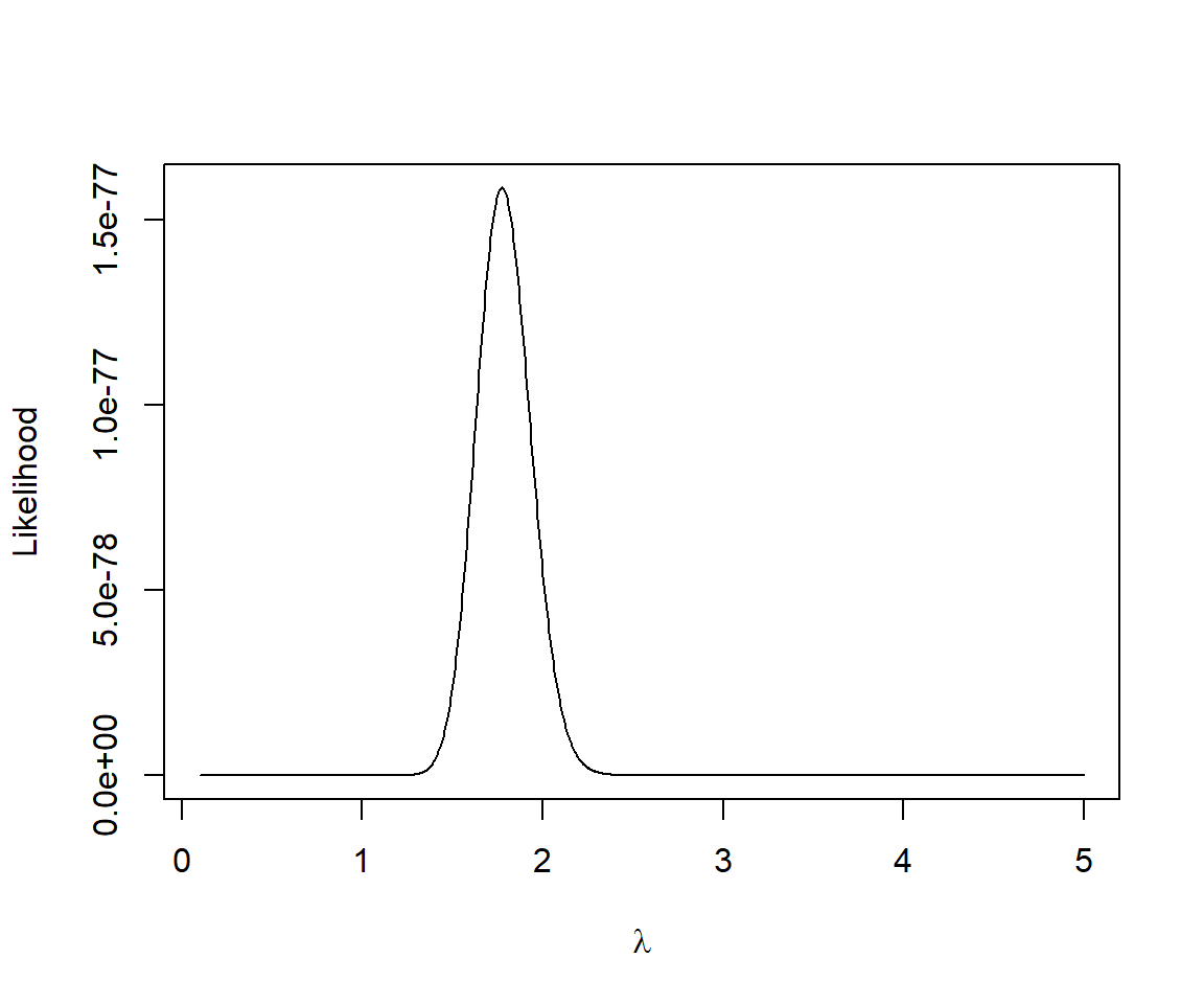

Figure 10.3: Likelihood of the slug data as a function of $\lambda$, assuming the slug counts are Poisson distributed with constant $\lambda$.

We can find the value of value of $\lambda$ that makes the likelihood of our data as large as possible using the which.max function in R⁸:

# lambda that maximizes the likelihood
lambda.test[which.max(L.vals)]

[1] 1.772573

This value is identical to the sample mean out to 2 decimal places (we could get a more accurate answer if we used a finer grid).

As previously mentioned, the likelihood values are really small for all values of $\lambda$. This can lead to numerical challenges associated with representing small numbers (referred to as underflow), making it difficult to find the parameters that maximize the likelihood. Therefore, it is more common to work with the log-likelihood, which will be maximized at the same value of $\lambda$. To verify, we create a function for calculating the log-likelihood of the data and repeat our grid search. We will again use the dpois function, but we add the argument log = TRUE so that this function returns $\log (f(y_i;\lambda ))$ rather than $f(y_i;\lambda )$. In addition, we sum the individual terms (using the sum function) rather than taking their product. Instead of writing another loop, we will take advantage of the map_dbl function in the purrr library to calculate the log-likelihood values:

#log Likelihood
logL.s<-function(lambda, dat){
     sum(dpois(dat,lambda, log = TRUE))
}
# evaluate at the same grid of lambda values
logL.vals <- purrr::map_dbl(lambda.test, logL.s, dat=slugs$slugs)

# find the value that maximizes the log L and plot
lambda.test[which.max(logL.vals)]

[1] 1.772573

We see that the same value of $\lambda$ = 1.77 maximizes both the likelihood and log-likelihood (Figure 10.4).

plot(lambda.test, logL.vals, xlab=expression(lambda), ylab="Log Likelihood",type="l")
abline(v=lambda.test[which.max(logL.vals)])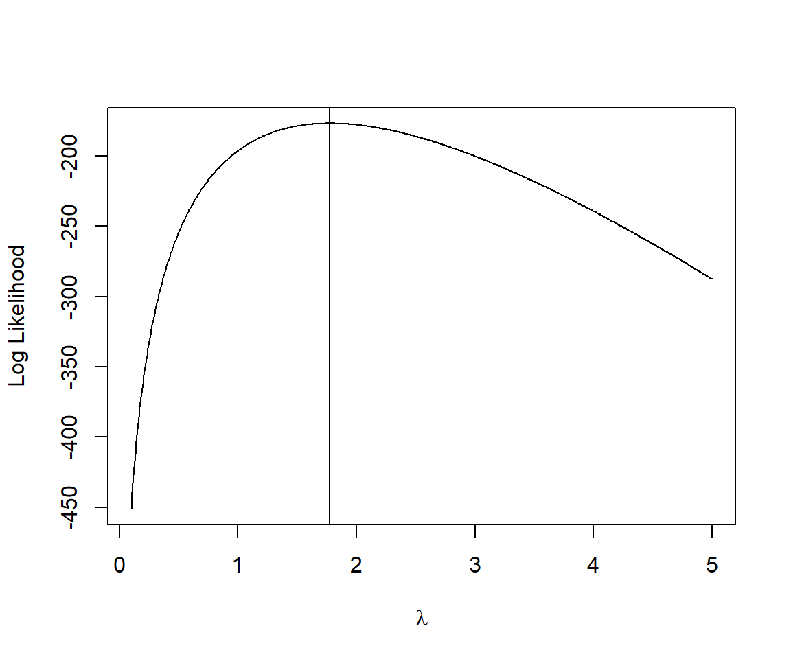

Figure 10.4: Log-likelihood of the slug data as a function of $\lambda$, assuming the slug counts are Poisson distributed with constant $\lambda$.

10.5.3 Using numerical optimizers

Most software packages have built in functions that can find parameter values that either maximize or minimize a specified function. R has several functions available for this purpose, including optim, nlm, nlminb, among others. In this section, we will explore the use of optim, which can be used to find the parameters that minimize any function. It has the following arguments that we must supply:

• par = a vector of “starting” parameters (first guesses).

• fn = a function to minimize. Importantly, the first argument of this function must correspond to the vector of parameters that we want to optimize (i.e., estimate).

These two arguments are expected to occur in this order with par first and fn second. But, as with any function in R, we can change the order of the arguments as long as we use their names. Consider, for example, dpois. Its first two arguments are x and lambda. Normally, I am lazy and just pass the arguments in this order without supplying their names. For example,

dpois(3, 5)

[1] 0.1403739

We can, however, reverse the order if we use the argument names:

dpois(lambda = 5, x = 3)

[1] 0.1403739

We can use the method argument to specify a particular optimization method (we will use method = "BFGS"). We can also pass other arguments to optim (e.g., dat, which is needed to calculate the value of the log-likelihood). Importantly, by default, optim tries to find a minimum. Thus, we create a new function, minus.logL.s that calculates the negative log-likelihood. The value that minimizes the negative log-likelihood will maximize the log-likelihood.

minus.logL.s <- function(lambda, dat){
   -sum(dpois(dat,lambda, log = TRUE))
}

Most numerical optimization routines are iterative. They begin with a starting value (or guess), and then use information about the function (and its derivatives) at that guess to derive the next value to try. This results in a sequence of iterative guesses that hopefully converge to the true minimum. If there is only 1 minimum (or maximum), most optimizers will work well. But, if there are multiple minima or maxima, then optimizers will often converge to the one closest to the starting value. Thus, it can be important to try different starting values to help determine if there are multiple minima. If you find that the results from using optim depend on the starting value, then you should be cautious, try multiple starting values, and select the one that results in the smallest negative log-likelihood. You might also consider trying alternative estimation approaches (e.g., Bayesian methods that rely on Monte Carlo Markov Chain [MCMC] sampling may be more robust; Lele, Dennis, and Lutscher 2007)

For the slug example, there is only 1 minimum (Figure 10.3, Figure 10.4), and therefore, most starting values for $\lambda$ will converge to the correct value (though, we must supply a starting value > 0 since $\lambda >0$ in the Poisson distribution). Here, we supply a value of 2 to begin the optimization routine:

mle.fit<-optim(par = 2, fn = minus.logL.s,  method = "BFGS",  dat = slugs$slugs)  

Warning in dpois(dat, lambda, log = TRUE): NaNs produced

Note that optim outputs a warning here about NaNs being produced. The parameter, $\lambda$ of the Poisson distribution, has to be positive. We have not told optim this, and therefore, it is possible that it will try negative values when attempting to evaluate the log-likelihood. In this case, dpois will return an NaN, giving us the warning. Yet, if we inspect the output, we will see that it was able to continue and find the value of $\lambda$ that maximizes the likelihood:

mle.fit 

$par
[1] 1.775

$value
[1] 176.8383

$counts
function gradient 
      15        6 

$convergence
[1] 0

$message
NULL

We see that optim returns:

• par = the value of $\lambda$ that minimizes the negative log-likelihood; this is the maximum likelihood estimate!
• value = the value of the function (i.e., the negative log-likelihood) at its minimum value
• counts = information about how hard it had to work to find the minimum. We see that it had to calculate the likelihood for 15 different values of $\lambda$ and it calculated $\frac{d\log L}{d\lambda }$ 6 times (function and gradient, respectively)
• convergence = an indicator of whether the optimizer converged; a value of 0 suggests the optimizer was successful, whereas a value of 1 would indicate that it hit a limit based on the maximum number of iterations allowed (which can be changed from a default value of 100)

In summary, we have used 3 different methods for finding the value of $\lambda$ that maximizes the log-likelihood. In each case, we ended up with $\hat{\lambda }=1.77$.

10.5.4 Fitting the alternative data-generating model (site-specific Poisson distributions)

Consider our alternative data-generating model:

$Y_{ij}\sim Poisson({\lambda }_j)$ where $i=1,2,\dots ,40$ and $j=1,2$ for the Nursery and Rookery site, respectively.

We could estimate ${\lambda }_1$ and ${\lambda }_2$ in a number of different ways. We could split the data by field and then use each of the methods previously covered (calculus, grid search, numerical optimizer) but applied separately to each data set. Nothing new there. We could apply a 2-dimensional grid search, which could be instructive for other situations where we have more than 1 parameter (e.g., when fitting a negative binomial data-generating model to the data). Or, we could continue to get familiar with optim as it offers a more rigorous way of finding parameters that maximize the likelihood and will also facilitate estimation of parameter uncertainty, as we will see later. Using optim will require rewriting our negative log-likelihood function to allow for two parameters. We will also need to pass to the function the data that identifies from which field the observations come from so that it uses the correct $\lambda$ for each observation. One option is given below, where we now pass a full data set rather than just the slug counts:

minus.logL.2a<-function(lambdas, dat){
     -sum(dpois(dat$slugs[dat$field=="Nursery"], lambdas[1], log=TRUE))-
      sum(dpois(dat$slugs[dat$field=="Rookery"], lambdas[2], log=TRUE))
  }

Earlier, we noted that we did not tell optim that our parameters must be > 0 (i.e., ${\lambda }_1,{\lambda }_2>0$). We could use a different optimizer that allows us to pass constraints on the parameters. For example, we could change to method = "L-BFGS-B" and supply a lower bound for both parameters via an extra argument, lower = c(0, 0). Alternatively, we could choose to specify our likelihood in terms of parameters estimated on the log-scale and then exponentiate these parameters to get $\hat{\lambda }$. This is often a useful strategy for constraining parameters to be positive. For example, we could use:

minus.logL.2b<-function(log.lambdas, dat){
     -sum(dpois(dat$slugs[dat$field=="Nursery"], exp(log.lambdas[1]), log=TRUE))-
      sum(dpois(dat$slugs[dat$field=="Rookery"], exp(log.lambdas[2]), log=TRUE))
  }

In this way, we estimate parameters that can take on any value between $-\mathrm{\infty }$ and $\mathrm{\infty }$, but the parameters used in dpois will be > 0 because we exponentiate the optimized parameters using exp(). In fact, this is what R does when it fits the Poisson model using its built in glm function.

Let’s use optim with minus.logL.2b to estimate ${\lambda }_1$ and ${\lambda }_2$ in our alternative data-generating model (note, you will need to supply a vector of starting values when using optim, say par = c(2,2)).

mle.fit.2lambdas <- optim(par = c(2, 2), fn = minus.logL.2b, dat = slugs, method = "BFGS")  
mle.fit.2lambdas 

$par
[1] 0.2429461 0.8219799

$value
[1] 171.1275

$counts
function gradient 
      29       10 

$convergence
[1] 0

$message
NULL

Remember, our parameters now reflect $\log (\lambda )$, so to estimate $\lambda$, we have to exponentiate these values:

exp(mle.fit.2lambdas$par)

[1] 1.275 2.275

These are equivalent to the sample means in the two fields:

slugs %>% group_by(field) %>%
  dplyr::summarize(mean(slugs))

# A tibble: 2 × 2
  field   `mean(slugs)`
  <chr>           <dbl>
1 Nursery          1.27
2 Rookery          2.28

At this point, to test your understanding, you might consider the following two exercises:

Exercise: modify the likelihood function to fit a model assuming the slug counts were generated by a negative binomial distribution (ecological version; Section 9.10.6.2).

Exercise: modify the two parameter Poisson model so that it is parameterized using reference coding. Your estimates should match those below:

glm(slugs~field, data=slugs, family=poisson())

Call:  glm(formula = slugs ~ field, family = poisson(), data = slugs)

Coefficients:
 (Intercept)  fieldRookery  
      0.2429        0.5790  

Degrees of Freedom: 79 Total (i.e. Null);  78 Residual
Null Deviance:      224.9 
Residual Deviance: 213.4    AIC: 346.3

10.6 Properties of maximum likelihood estimators

Let $\theta$ be a parameter of interest and $\hat{\theta }$ be the maximum likelihood estimator of $\theta$. Maximum likelihood estimators (MLEs) have many desirable properties (assuming the choice of distribution is correct). In particular,

• MLEs are consistent, meaning that as the sample size increases towards $\mathrm{\infty }$, they will converge to the true parameter value.
• MLEs are asymptotically unbiased, i.e., $E(\hat{\theta })\to \theta$ as $n\to \mathrm{\infty }$. Maximum likelihood estimators are not, however, guaranteed to be unbiased in small samples. As one example, the maximum likelihood estimator of ${\sigma }^2$ for Normally distributed data is given by ${\hat{\sigma }}_{MLE}^2=\sum _{i=1}^n(y_i-\overline{y}{)}^2/n$, which has as its expected value, $E[{\hat{\sigma }}_{MLE}^2]=\frac{n-1}{n}{\sigma }^2$. The bias of the maximum likelihood estimator becomes negligible as sample sizes become large. In cases like this where you can derive, analytically, an expression for bias, you can form an unbiased estimator that may perform better in small samples. For example, you may be familiar with the unbiased estimator, ${\hat{\sigma }}^2=\sum _{i=1}^n(y_i-\overline{y}{)}^2/(n-1)$.
• MLEs will have the minimum variance among all estimators as $n\to \mathrm{\infty }$.

In addition, for large sample sizes, we can approximate the sampling distribution of maximum likelihood estimators using:

$$\hat{\theta }\sim N(\theta ,I^{-1}(\theta )),$$ where $I(\theta )$ is called the Information matrix. We will use this last property repeatedly as it provides the basis for constructing hypothesis tests and confidence intervals for maximum likelihood estimators.

Before we can define the Information matrix, we will need to formally define a Hessian; the Hessian is a matrix of second-order partial derivatives of a function, in this case, derivatives of the log-likelihood function with respect to the parameters $({\theta }_1,{\theta }_2,\dots ,{\theta }_p)$:

$$\text{Hessian}(\theta {)}_{p\times p}=\left[\begin{array}{cccc}\frac{{\partial }^{2}logL(\theta )}{\partial {\theta }_1^2}& \frac{{\partial }^{2}logL(\theta )}{\partial {\theta }_1{\theta }_2}& \cdots & \frac{{\partial }^{2}logL(\theta )}{\partial {\theta }_1{\theta }_p}\\ \frac{{\partial }^{2}logL(\theta )}{\partial {\theta }_1{\theta }_2}& \frac{{\partial }^{2}logL(\theta )}{\partial {\theta }_2^2}& \cdots & \frac{{\partial }^{2}logL(\theta )}{\partial {\theta }_2{\theta }_p}\\ ⋮& ⋮& \ddots & ⋮\\ \frac{{\partial }^{2}logL(\theta )}{\partial {\theta }_1{\theta }_p}& \frac{{\partial }^{2}logL(\theta )}{\partial {\theta }_2{\theta }_p}& \cdots & \frac{{\partial }^{2}logL(\theta )}{\partial {\theta }_p^2}\end{array}\right]$$

If there is only 1 parameter in the likelihood, then the Hessian will be a scaler and equal to $\frac{d^2\log L(\theta )}{d{\theta }^2}$, i.e., the second derivative of the log-likelihood with respect to the parameter.

The information matrix is defined in terms of the Hessian and takes one of two forms:

• The observed information matrix is the negative of the Hessian evaluated at the maximum likelihood estimate:

$${\text{observed }I(\theta {)}_{p\times p}=-\left[\begin{array}{cccc}\frac{{\partial }^{2}logL(\theta )}{\partial {\theta }_1^2}& \frac{\partial logL(\theta )}{\partial {\theta }_1{\theta }_2}& \cdots & \frac{{\partial }^{2}logL(\theta )}{\partial {\theta }_1{\theta }_p}\\ \frac{{\partial }^{2}logL(\theta )}{\partial {\theta }_1{\theta }_2}& \frac{{\partial }^{2}logL(\theta )}{\partial {\theta }_2^2}& \cdots & \frac{{\partial }^{2}logL(\theta )}{\partial {\theta }_2{\theta }_p}\\ ⋮& ⋮& \ddots & ⋮\\ \frac{{\partial }^{2}logL(\theta )}{\partial {\theta }_1{\theta }_p}& \frac{{\partial }^{2}logL(\theta )}{\partial {\theta }_2{\theta }_p}& \cdots & \frac{{\partial }^{2}logL(\theta )}{\partial {\theta }_p^2}\end{array}\right]|}_{\theta =\hat{\theta }}$$

• The expected information matrix is given by the expected value of the negative of the Hessian evaluated at the maximum likelihood estimate:

$${\text{expected }I(\theta {)}_{p\times p}=-E\left[\begin{array}{cccc}\frac{{\partial }^{2}logL(\theta )}{\partial {\theta }_1^2}& \frac{\partial logL(\theta )}{\partial {\theta }_1{\theta }_2}& \cdots & \frac{{\partial }^{2}logL(\theta )}{\partial {\theta }_1{\theta }_p}\\ \frac{{\partial }^{2}logL(\theta )}{\partial {\theta }_1{\theta }_2}& \frac{{\partial }^{2}logL(\theta )}{\partial {\theta }_2^2}& \cdots & \frac{{\partial }^{2}logL(\theta )}{\partial {\theta }_2{\theta }_p}\\ ⋮& ⋮& \ddots & ⋮\\ \frac{{\partial }^{2}logL(\theta )}{\partial {\theta }_1{\theta }_p}& \frac{{\partial }^{2}logL(\theta )}{\partial {\theta }_2{\theta }_p}& \cdots & \frac{{\partial }^{2}logL(\theta )}{\partial {\theta }_p^2}\end{array}\right]|}_{\theta =\hat{\theta }}$$

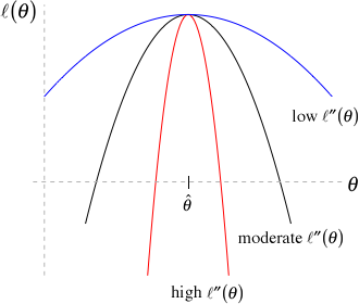
Note that the Hessian describes the curvature of the log-likelihood surface – the higher the curvature, the more quickly the log-likelihood decreases as we move away from the maximum likelihood estimate (Figure 10.5). If the curvature is large, then the asymptotic variance of $\hat{\theta }$ will be small. By contrast, when $\left[\frac{{\partial }^{2}logL(\theta )}{\partial {\theta }^2}\right]$ is close to 0, this suggests that the log-likelihood is “flat” with many different parameter values giving similar log-likelihoods. In this case, the inverse of the Hessian, and hence the variance, will be large.

Figure 10.5: Large values of the Hessian (red) correspond to high levels of Information, high curvature of the log-likelihood surface, and low levels of uncertainty. Figure from Jack Weiss’s online course notes.

Importantly, the Hessian is often used by numerical optimization methods (e.g., optim) to find parameter values that minimize an objective function (e.g., the negative log-likelihood). We can ask optim to return the Hessian by supplying the argument hessian = TRUE, which will be equivalent to the observed information matrix (since we defined our function as the negative of the log-likelihood, the minus sign will already be taken care of). We can then calculate the asymptotic variance-covariance matrix of $\hat{\theta }$ by taking the inverse of the Hessian.

Let’s demonstrate with our slug example, where we fit the alternative data-generating model that assumed separate Poisson distributions for each field. We begin by asking optim to return the Hessian by supplying an extra argument, hessian = TRUE:

mle.fit.2lambdas <- optim(par = c(2, 2), 
                          fn = minus.logL.2b, 
                          dat = slugs, 
                          method = "BFGS", 
                          hessian = TRUE)  
mle.fit.2lambdas 

$par
[1] 0.2429461 0.8219799

$value
[1] 171.1275

$counts
function gradient 
      29       10 

$convergence
[1] 0

$message
NULL

$hessian
              [,1]          [,2]
[1,]  5.100001e+01 -1.421085e-08
[2,] -1.421085e-08  9.100001e+01

We can calculate asymptotic standard errors for our parameters by finding the inverse of the Hessian. To find the inverse of a matrix, $H$, in R, we can use solve(H). Thus, we can find the variance/covariance matrix associated with parameter estimates using:

(var.cov.lambda <- solve(mle.fit.2lambdas$hessian))

             [,1]         [,2]
[1,] 1.960784e-02 3.062023e-12
[2,] 3.062023e-12 1.098901e-02

The diagonal elements of this matrix correspond to our estimates of the variance of our parameters; the square root of the diagonals thus give us their standard errors⁹

sqrt(diag(var.cov.lambda))

[1] 0.1400280 0.1048285

The off diagonals of our variance-covariance matrix tell us about how our parameters covary in their sampling distribution (i.e., do high values for ${\hat{\lambda }}_1$ tend to occur with high or low values of ${\hat{\lambda }}_2$). In this simple model, the parameter estimates are independent (data from the Nursery field does not inform the estimate of $\lambda$ for the Rookery field and data from the Rookery field do not inform our estimate of $\lambda$ for the Nursery field). If instead, we fit the model using effects coding, we will see that our parameters will covary in their sampling distribution.

Lastly, we can compare our estimates and their standard errors to those that are returned from R’s glm function, which we will see in Chapter 15:

summary(glm(slugs ~ field -1, data = slugs, family = "poisson"))

Call:
glm(formula = slugs ~ field - 1, family = "poisson", data = slugs)

Coefficients:
             Estimate Std. Error z value Pr(>|z|)    
fieldNursery   0.2429     0.1400   1.735   0.0827 .  
fieldRookery   0.8220     0.1048   7.841 4.46e-15 ***
---
Signif. codes:  0 '***' 0.001 '**' 0.01 '*' 0.05 '.' 0.1 ' ' 1

(Dispersion parameter for poisson family taken to be 1)

    Null deviance: 263.82  on 80  degrees of freedom
Residual deviance: 213.44  on 78  degrees of freedom
AIC: 346.26

Number of Fisher Scoring iterations: 6

We see that we have obtained exactly the same estimates and standard errors as reported by the glm function. Also, note that at the bottom of the summary output, we see Number of Fisher Scoring iterations: 6. This comparison highlights:

1. glm is fitting a model parameterized in terms of the log mean (i.e., log $\lambda$)
2. glm is using numerical routines similar to optim and also reports standard errors that rely on the asymptotic results discussed in the above section, namely, $\hat{\theta }\sim N(\theta ,I^{-1}(\theta ))$.

10.7 A more complicated example: Fitting a weight-at-age model

Let us now return to our motivating example involving a weight-at-age model for female black bears in Minnesota. We will use optim to fit the following model:

$$\begin{array}{r}Weigh{t}_i\sim N({\mu }_i,{\sigma }_i^2)\\ {\mu }_i=L_{\mathrm{\infty }}(1-e^{-K(Ag{e}_i-t_0)})\\ {\sigma }_i^2={\sigma }^2{\mu }_i^{2\theta }\end{array}$$

This allows us to model the mean using the von Bertalanffy growth function and model the variability about this mean using the variance function from Section 5.5.3.

We begin by constructing the likelihood function with the following parameters $L_{\mathrm{\infty }},K,t_0,\log (\sigma ),\theta$:

logL<-function(pars, dat){
    linf <- pars[1]  
    k <- pars[2]
    t0 <- pars[3]
    sig <- exp(pars[4])
    theta <- pars[5] 
    mu<-linf*(1 - exp(-k*(dat$age - t0))) 
    vari<-sig^2*abs(mu)^(2*theta)
    sigi<-sqrt(vari)
    ll<- -sum(dnorm(dat$wtkg, mean = mu, sd = sigi, log = T))
    return(ll) 
  }   

To get starting values, which we denote using a superscript $s$, we revisit our plot of the data (Figure 10.1), noting:

• The smooth curve asymptotes at around 100, so we use $L_{\mathrm{\infty }}^s=100$
• $K$ tells us how quickly we approach this asymptote as bears age. If we set $\mu =L_{\mathrm{\infty }}/2$ and solve for $K$, this gives $K=log(2)/(t-t_0)$. Then, noting that $\mu$ appears to be at $L_{\mathrm{\infty }}$/2 = 50 at around 3 years of age, we set $K^s=log(2)/3=0.23$
• $t_0$ is the x-intercept (i.e., the Age at which $\mu =0$); an extrapolation of the curve to $x=0$ suggests that $t_0$ should be slightly less than 0, say $t_0^s=-0.1$
• Most of the residuals when age is close to 0 are within approximately $\pm 10$ kg. For Normally distributed data, we expect 95% of the observations to be within $\pm 2\sigma$ so we set $\log (\sigma {)}^s=log(10/2)=1.61$
• We set ${\theta }^0$ = 1 (suggesting the variance increases linearly with the mean)

fitvb <- optim(par = c(100, 0.23, -0.1, 1.62, 1), 
               fn = logL,dat = beargrowth, 
               method = "BFGS", hessian = TRUE)
fitvb

$par
[1] 87.1070613  0.2853005  0.1530582 -0.1744772  0.6607753

$value
[1] 2156.353

$counts
function gradient 
     108       25 

$convergence
[1] 0

$message
NULL

$hessian
           [,1]       [,2]        [,3]        [,4]       [,5]
[1,]   1.633524   200.5033   -31.11917    8.632616    33.2212
[2,] 200.503252 36487.7264 -7444.52556 1325.372227  4676.6273
[3,] -31.119171 -7444.5256  2101.48826 -271.183081  -841.5901
[4,]   8.632616  1325.3722  -271.18308 1138.010281  4383.5226
[5,]  33.221200  4676.6273  -841.59012 4383.522578 17355.9438

Let’s inspect the fit of our model by adding our predictions from the model to our data set (Figure 10.6).

pars<-data.frame(Linf = fitvb$par[1], K = fitvb$par[2], t0 = fitvb$par[3],
                 sigma = exp(fitvb$par[4]), theta = fitvb$par[5])
beargrowth <- beargrowth %>% 
  mutate(mu.hat = pars$Linf*(1 - exp(-pars$K*(age - pars$t0))))
ggplot(beargrowth, aes(age, wtkg)) + 
  geom_point() + geom_line(aes(age, mu.hat), col = "red", linewidth = 1) +
  ylab("Weight (kg)") + xlab("Age (years)") +
  theme_bw()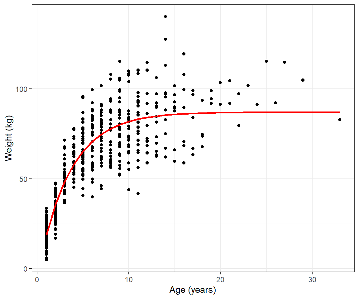

Figure 10.6: Fitted von Bertalanffy growth curve to weight-at-age data for black bears in Minnesota.

Next, let’s create and inspect plots using standardized residuals (Figure 10.7). In particular, we can plot standardized residuals versus fitted values to evaluate whether the von Bertalanffy growth curve adequately describes how the mean weight varies with age. We can also plot the sqrt root of absolute values of these residuals versus fitted values to evaluate whether our variance model is appropriate.

beargrowth <- beargrowth %>%
  mutate(sig.hats = pars$sigma^2*abs(mu.hat)^(2*pars$theta)) %>%
  mutate(stdresids = (wtkg - mu.hat)/(sig.hats),
         sqrt.abs.resids = sqrt(abs(stdresids)))
p1<-ggplot(beargrowth, aes(mu.hat, stdresids)) + geom_point() + 
  geom_hline(yintercept=0) + geom_smooth() + theme_bw()
p2<-ggplot(beargrowth, aes(mu.hat, sqrt.abs.resids)) + geom_point() + 
   geom_smooth() + theme_bw()
p1+p2

`geom_smooth()` using method = 'loess' and formula = 'y ~ x'
`geom_smooth()` using method = 'loess' and formula = 'y ~ x'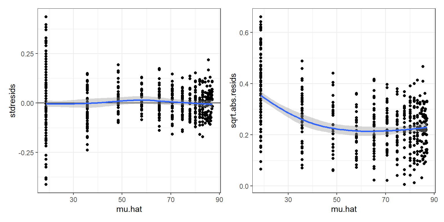

Figure 10.7: Standardized residuals (left panel) and square-rooted absolute values of these residuals (right panel) versus fitted values from the von Bertalanffy growth model applied to weight-at-age data from black bears in Minnesota.

The standardized residuals do not exhibit any trend as we move from left to right in the residual versus fitted value plot (left panel of Figure 10.7), but residuals of the smallest bears appear to be slightly more variability (right panel of Figure 10.7). At this point, we could try to fit alternative growth models for the mean weight at age or alternative models for the variance about the mean to see if we could better match the data. Nonetheless, the fit of the von Bertalanffy growth curve (Figure 10.6) provides a nice summary of the weight-at-age relationship. What if we wanted to add confidence or prediction intervals to our plot?

10.8 Confidence intervals for functions of parameters

The results from Section 10.6 provide a way for us to calculate uncertainty associated with our model parameters. I.e., if we let $\hat{\mathrm{\Psi }}=({\hat{L}}_{\mathrm{\infty }},\hat{K},{\hat{t}}_0,\widehat{\log (\sigma )},\hat{\theta })$, then we know the asymptotic variance-covariance matrix of $\hat{\mathrm{\Psi }}$ is given by $I^{-1}(\mathrm{\Psi })$, which we can estimate from the returned Hessian:

(vcov.psi <- solve(fitvb$hessian))

             [,1]          [,2]          [,3]          [,4]          [,5]
[1,]  2.737807861 -2.424357e-02 -0.0455615458  0.0052606707 -2.245891e-03
[2,] -0.024243567  3.165257e-04  0.0007662437  0.0001665308 -4.378909e-05
[3,] -0.045561546  7.662437e-04  0.0025635157  0.0016454637 -4.105409e-04
[4,]  0.005260671  1.665308e-04  0.0016454637  0.0346870394 -8.735923e-03
[5,] -0.002245891 -4.378909e-05 -0.0004105409 -0.0087359227  2.260206e-03

The diagonals of this matrix tell us about the expected variability of our parameter estimates (across repetitions of data collection and analysis), with the square root of these elements giving us our standard errors. Thus, we can form 95% confidence intervals for our model parameters using the assumption that the sampling distribution is Normal. For example, a 95% confidence interval for $L_{\mathrm{\infty }}$ is given by:

SE.Linf<-sqrt(diag(vcov.psi))[1]
fitvb$par[1] + c(-1.96, 1.96)*rep(SE.Linf,2)

[1] 83.86398 90.35014

All good, but again, what if we want a confidence interval for $E[Y_i|Ag{e}_i]={\mu }_i=L_{\mathrm{\infty }}(1-e^{-K(Ag{e}_i-t_0)})$, which is a function of more than 1 of our parameters. To quantify the uncertainty associated with $E[Y_i|Ag{e}_i]$, we have to consider the variability associated with each parameter. We also have to consider how the parameters covary – i.e., we need to consider the off-diagonal elements of $I^{-1}(\hat{\mathrm{\Psi }})$. For example, the (2, 1) element of $I^{-}(\hat{\mathrm{\Psi }})$ is negative, suggesting that large estimates of $L_{\mathrm{\infty }}$ tend to be accompanied by small estimates of $K$ and vice versa.

Recall, in Chapter 5, we learned how to use matrix multiplication to get predicted values and their variance for linear models, possibly with non-constant variance. We briefly review those results here. Recall, if $\hat{\beta }\sim N(\beta ,\mathrm{\Sigma })$, then:

$$X\hat{\beta }\sim N(X\beta ,X\mathrm{\Sigma }{X}^T),$$ and we can estimate the mean and variance using matrix multiplication, replacing $\beta$ with $\hat{\beta }$ and $\mathrm{\Sigma }$ with $\hat{\mathrm{\Sigma }}$, where $\hat{\mathrm{\Sigma }}$ is the estimated variance covariance matrix of $\hat{\beta }$. This works if we are interested in a linear combination of our parameters (i.e., a weighted sum). But, what if we are interested in non-linear functions of parameters? I.e., $E[Y_i|Ag{e}_i]=L_{\mathrm{\infty }}(1-e^{-k(Ag{e}_i-t_0)})$. We have 3 options:

• Use a bootstrap (see Chapter 2)
• Use the Delta method, which we will see shortly
• Switch to Bayesian inference and use posterior distributions

10.8.1 Delta Method

To understand how the delta method is derived, you have to know something about Taylor’s series approximations. Taylor’s series approximations are incredibly useful (e.g., they also serve to motivate some of the numerical methods we have used, including the BFGS method implemented by optim). We won’t get into the gory details here, but rather will focus on implementation. To implement the delta method, we need to be able to take derivatives of our function with respect to each of our parameters.

Let $f(L_{\mathrm{\infty }},K,t_0,\log (\sigma ),\theta ;Age)=L_{\mathrm{\infty }}(1-e^{-K(Age-t_0)})$ be our function of interest (i.e., the mean weight at a given age). To calculate $Var[f({\hat{L}}_{\mathrm{\infty }},\hat{K},{\hat{t}}_0,\log (\hat{\sigma }),\hat{\theta };Age)]$, we need to determine:

$f^{\prime }(L_{\mathrm{\infty }},K,t_0,\log (\sigma ),\theta ;Age)=(\frac{\partial \mu }{\partial L_{\mathrm{\infty }}},\frac{\partial \mu }{\partial K},\frac{\partial \mu }{\partial t_0},\frac{\partial \mu }{\partial \log (\sigma )},\frac{\partial \mu }{\partial \theta })$

Then, we can approximate the variance of $f({\hat{L}}_{\mathrm{\infty }},\hat{K},{\hat{t}}_0,\log (\hat{\sigma }),\hat{\theta };Age)=\hat{E}[Y_i|Ag{e}_i]$ for $Ag{e}_i$ using matrix multiplication:

$$\hat{E}[Y_i|Ag{e}_i]\approx f^{\prime }(L_{\mathrm{\infty }},K,t_0,\log (\sigma ),\theta )I^{-1}(\mathrm{\Psi })f^{\prime }(L_{\mathrm{\infty }},K,t_0,\log (\sigma ),\theta {)}^T{|}_{L_{\mathrm{\infty }}={\hat{L}}_{\mathrm{\infty }},K=\hat{K},t_0={\hat{t}}_0,\log (\sigma )=\log (\hat{\sigma }),\theta =\hat{\theta }}$$

Because our function does not involve $\log (\sigma )$ or $\theta$, we can simplify things a bit and just work with $f^{\prime }(L_{\mathrm{\infty }},K,t_0)$ and the first 3 rows and columns of $I^{-1}(\mathrm{\Psi })$¹⁰:

• $\frac{\partial \mu }{\partial L_{\mathrm{\infty }}}=(1-e^{-K(Age-t_0)})$

• $\frac{\partial \mu }{\partial K}=L_{\mathrm{\infty }}(Age-t_0)e^{-K(Age-t_0)}$

• $\frac{\partial \mu }{\partial t_0}=-L_{\mathrm{\infty }}K{e}^{-K(Age-t_0)})$

To calculate the variance for a range of ages (e.g., $Age=1,2,...,35$), we create a 35 x 3 dimension matrix with a separate row for each $Age$ and the columns giving $f^{\prime }$ for each $Age$:

age <- 1:35
mu.hat <- pars$Linf*(1-exp(-pars$K*(age-pars$t0)))
fprime<-as.matrix(cbind(1-exp(-pars$K*(age-pars$t0)),
                         pars$Linf*(age-pars$t0)*exp(-pars$K*(age-pars$t0)),
                         -pars$Linf*pars$K*exp(-pars$K*(age-pars$t0))))

We then determine the variance using matrix multiplication, pulling off the diagonal elements (the off-diagonal elements hold the covariances between observations for different ages):

var.mu.hat <- diag(fprime %*% solve(fitvb$hessian)[1:3,1:3] %*%t(fprime))

Alternatively, the emdbook package (B. Bolker 2023) has a function, deltavar, that will do the calculations for you if you supply a function for calculating $f()$ (via argument meanval) and you pass the asymptotic variance covariance matrix, $I^{-1}(\mathrm{\Psi })$ (via the Sigma argument).

library(emdbook)
var.mu.hat.emd <- deltavar(linf*(1-exp(-k*(age-t0))), 
                      meanval=list(linf=fitvb$par[1], k=fitvb$par[2], t0=fitvb$par[3]), 
                      Sigma=solve(fitvb$hessian)[1:3,1:3])

We can take the square root of the diagonal elements of var.mu.hat to get SEs for forming pointwise confidence intervals for $E[Y_i|Ag{e}_i]$ at each Age.

muhats <- data.frame(age=age, 
                     mu.hat=mu.hat, 
                     se.mu.hat = sqrt(var.mu.hat))
ggplot(beargrowth, aes(age, wtkg)) + 
  geom_point() + geom_line(aes(age, mu.hat), col="red", size=1) +
  ylab("Weight (kg)") + xlab("Age (years)") + theme_bw() +
  geom_ribbon(data=muhats, aes(x=age, 
                                 ymin=mu.hat-1.96*se.mu.hat, 
                                 ymax=mu.hat+1.96*se.mu.hat),
                 inherit.aes = FALSE, fill = "blue", alpha=0.5)

Warning: Using `size` aesthetic for lines was deprecated in ggplot2 3.4.0.
ℹ Please use `linewidth` instead.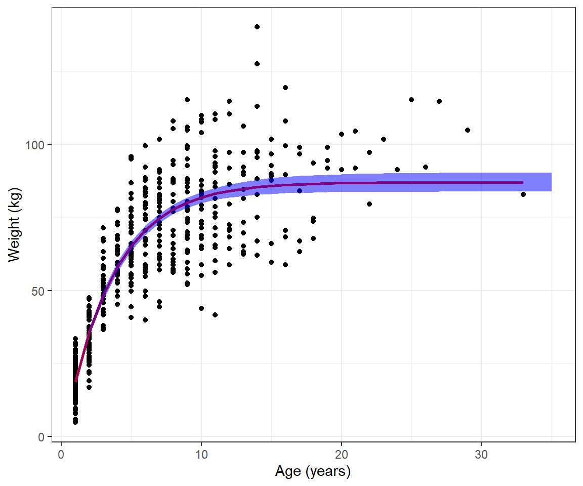

Figure 10.8: Fitted von Bertalanffy growth curve and 95% confidence interval estimated from weight-at-age data for black bears in Minnesota.

Lastly, we could calculate prediction intervals, similar to the example in Chapter 5 by adding +/- 2${\sigma }_i$, where ${\sigma }_i=\sqrt{{\sigma }^2{\mu }_i^{2\theta }}$ (Figure 10.9).

muhats <- muhats %>%
  mutate(pi.up = mu.hat + 1.95*se.mu.hat + 2*sqrt(pars$sigma^2*mu.hat^(2*pars$theta)),
         pi.low = mu.hat - 1.95*se.mu.hat - 2*sqrt(pars$sigma^2*mu.hat^(2*pars$theta)))
ggplot(beargrowth, aes(age, wtkg)) + 
  geom_point() + geom_line(aes(age, mu.hat), col="red", size=1) +
  ylab("Weight (kg)") + xlab("Age (years)") + theme_bw() +
  geom_ribbon(data=muhats, aes(x=age, 
                                 ymin=mu.hat-1.96*se.mu.hat, 
                                 ymax=mu.hat+1.96*se.mu.hat),
                 inherit.aes = FALSE, fill = "blue", alpha=0.2)+
  geom_ribbon(data=muhats, aes(x=age, 
                                 ymin=pi.low, 
                                 ymax=pi.up),
                 inherit.aes = FALSE, fill = "red", alpha=0.2)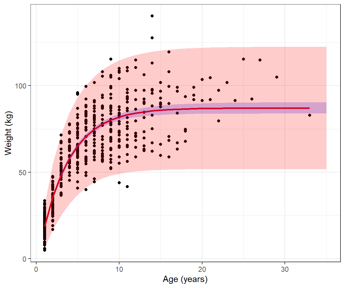

Figure 10.9: Fitted von Bertalanffy growth curve and 95% confidence and prediction intervals estimated from weight-at-age data for black bears in Minnesota.

10.9 Likelihood ratio test

A likelihood ratio test can be used to compare nested models with the same probability generating mechanism (i.e., same statistical distribution for the response variable). Parameters must be estimated using maximum likelihood, and we must be able to get from one model to the other by setting a subset of the parameters to specific values (typically 0).

In our slug example, we could use a likelihood ratio test to compare the following 2 models:

Model 1:

• $Y_{ij}\sim Poisson({\lambda }_j)$ with $j=1$ for the Nursery and $j=2$ for the Rookery.

Model 2:

• $Y_i\sim Poisson(\lambda )$ (i.e., ${\lambda }_2={\lambda }_1$)

The test statistic in this case is given by:

$LR=2\log \left[\frac{L({\lambda }_1,{\lambda }_2;Y)}{L(\lambda ;Y)}\right]=2[\log L({\lambda }_1,{\lambda }_2;Y)-\log L(\lambda ;Y)]$

Asymptotically, the sampling distribution of the likelihood ratio test statistic is given by a ${\chi }^2$ distribution with degrees of freedom equal to the difference in the number of parameters in the two models (i.e., df = 1 in our case). We can easily implement this test using the output from optim (recall that the negative log-likelihood values at the maximum likelihood estimates are stored in the value slot of mle.fit.2lambdas and mle.fit):

(LR<-2*(-mle.fit.2lambdas$value + mle.fit$value))

[1] 11.42156

This gives us a test statistic. To calculate a p-value, we need to compute the probability of obtaining a test statistic this large or larger, if the null hypothesis is true. If the null hypothesis is true, then the likelihood ratio statistic approximately follows a ${\chi }^2$ distribution with 1 degree of freedom. The p-value for a ${\chi }^2$ test is always calculated using the right tail of the distribution. We can use the pchisq function to calculate this probability:

1-pchisq(LR, df=1); # or

[1] 0.0007259673

pchisq(LR, df=1, lower.tail = FALSE)

[1] 0.0007259673

We can verify this result by comparing it to what we would get if we used the anova function in R to compare the two models:

full.glm<-glm(slugs~field, data=slugs, family=poisson())  
reduced.glm<-glm(slugs~1, data=slugs, family=poisson())
anova(full.glm, reduced.glm, test="Chisq")

Analysis of Deviance Table

Model 1: slugs ~ field
Model 2: slugs ~ 1
  Resid. Df Resid. Dev Df Deviance Pr(>Chi)    
1        78     213.44                         
2        79     224.86 -1  -11.422 0.000726 ***
---
Signif. codes:  0 '***' 0.001 '**' 0.01 '*' 0.05 '.' 0.1 ' ' 1

10.10 Profile likelihood confidence intervals

Typically, confidence intervals associated with maximum likelihood estimates are formed using the Normal approximation, $\hat{\theta }\sim N(\theta ,I^{-1}(\theta ))$. This will work well when our sample size is large but may fail to include the true parameter $(1-\alpha )$% of the time when $n$ is small and the log-likelihood surface is not symmetric. As an alternative, we can “invert” the likelihood-ratio test to get a profile likelihood-based confidence interval. Here, “inverting” the test means creating a confidence interval using the parameter values for which we would not reject the null hypothesis when conducting a likelihood ratio test. The confint function in R will calculate profile-likelihood based intervals by default for some models (e.g., mixed effect models fit using lmer; Chapter 18). Thus, it is a good idea to have some familiarity with this approach. Let’s demonstrate with a simple example, calculating a profile-likelihood based confidence interval for $\lambda$ in our null data-generating model.

A likelihood ratio test could be used to evaluate $H_0:\lambda ={\lambda }_0$ vs. $H_A:\lambda \ne {\lambda }_0$ for several different values of ${\lambda }_0$ (e.g., the values we created earlier when using a grid search to find the maximum likelihood estimator which we previously stored in an object called lambda.test). Our test statistic (Equation 10.6) would, in this case, compare the negative log-likelihoods when:

• $\lambda$ is set to the maximum likelihood estimator, $\hat{\lambda }$ (our unconstrained model)
• $\lambda$ is set to a specific value, ${\lambda }_0$ (our constrained model)

$$\begin{array}{}\text{(10.6)}& LR=2\log \left[\frac{L(\hat{\lambda }|Y)}{L({\lambda }_0|Y)}\right]\sim {\chi }_1^2\end{array}$$

We would reject $\lambda ={\lambda }_0$ at $\alpha =0.05$ if $LR>{\chi }_1^2(0.95)$, where ${\chi }_1^2(0.95)$ is the 95${}^{th}$ percentile of the ${\chi }_1^2$ distribution. We would fail to reject the null hypotheses if $LR<{\chi }_1^2(0.95)$. Values of $\lambda$ for which we would not reject the null hypothesis are plausible, given the data, and we will therefore want to include them in our confidence interval (Figure 10.10).

Figure 10.10: Profile-likelihood confidence interval for the single $\lambda$ model fit to the slug data. Figure derived from code originally posted by Jack Weiss for his Statistical Ecology course.

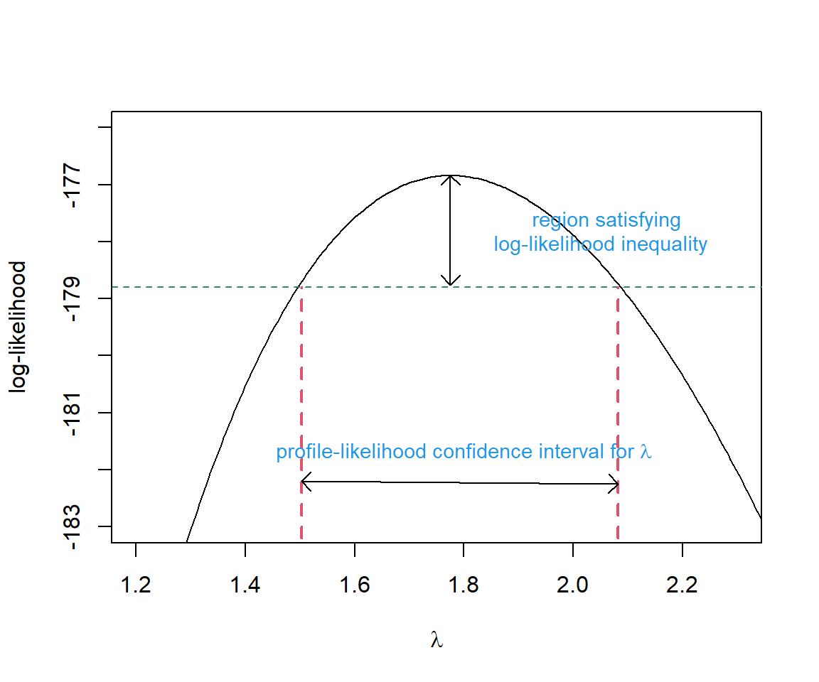
To calculate the profile likelihood confidence interval, remember that the negative log-likelihood value at the maximum likelihood estimate is stored as value in the output returned by optim (and specifically, for this problem, as mle.fit$value). In addition, we already calculated the log-likelihood for several values of ${\lambda }_0$ in Section 10.5.2. Thus, we just need to calculate twice the difference in log-likelihood values (using ${\hat{\lambda }}_{MLE}$ and ${\lambda }_0$) and identify the values of ${\lambda }_0$ where $LR<{\chi }_1^2(0.95)$.

 # finds all values of lambda that are not rejected by the hypoth test
ind<-I(2*(-mle.fit$value - logL.vals) < qchisq(0.95, df=1))
(CI.95<-range(lambda.test[ind]))

[1] 1.502803 2.081582

Let’s compare this interval to a Normal-based confidence interval. To do so, we need to repeat the optimization but request that optim also return the Hessian.

mle.fit <-   mle.fit<-optim(par = 2,
                            fn = minus.logL.s,  
                            method = "BFGS",  
                            dat = slugs$slugs, 
                            hessian = TRUE)

Warning in dpois(dat, lambda, log = TRUE): NaNs produced

SE<-sqrt(solve(mle.fit$hessian))
mle.fit$par + c(-1.96, 1.96)*rep(SE,2)

[1] 1.483049 2.066951

We see that, unlike the Normal-based interval, the profile likelihood interval is not symmetric and it includes slightly larger values of $\lambda$. Yet, the two confidence intervals are quite similar as might be expected given that the log-likelihood surface is nearly symmetric (Figure 10.10).

We can extend this basic idea to multi-parameter models, but calculating profile-likelihood-based confidence intervals becomes much more computationally intensive. In order to calculate a profile-likelihood confidence interval for a parameter in a multi-parameter model, we need to:

1. Consider a range of values associated with the parameter of interest (analogous to lambda.test in our simple example).
2. For each value in [1], we fix the parameter of interest and then determine maximum likelihood estimates for all other parameters (i.e., we need to optimize the likelihood several times, each time with the focal parameter fixed at a specific value).
3. We then use the likelihood-ratio test statistic applied to the likelihoods in [2] (our constrained model) and the likelihood resulting from allowing all parameters, including our focal parameter, to be estimated (our unconstrained model).

If we want to get confidence intervals for multiple parameters, we have to repeat this process for each of them. Alternatively, it is possible to calculate confidence regions for multi-parameter sets by considering more than 1 focal parameter at a time and a multi-degree-of-freedom likelihood-ratio ${\chi }^2$ test. See e.g., B. M. Bolker (2008) for further examples and discussion and the bbmle package for an implementation in R (B. Bolker and R Development Core Team 2020).

10.11 Aside: Least squares and maximum likelihood

It is interesting and sometimes useful to know that the least-squares and maximum likelihood are equivalent when data are Normally distributed. To see this connection, note that the likelihood for data that are Normally distributed is given by:

$L(\mu ,{\sigma }^2;y_1,y_2,\dots ,y_n)=\prod _{i=1}^n\frac{1}{\sqrt{2\pi }\sigma }{e}^{-\frac{(y_i-{\mu }_i{)}^2}{2{\sigma }^2}}$

With simple linear regression, we assume $Y_i\sim N({\mu }_i,{\sigma }^2)$ with ${\mu }_i={\beta }_0+X_i{\beta }_1$. Thus, we can write the likelihood as:

$L({\beta }_0,{\beta }_1,\sigma ;y_1,y_2,\dots ,y_n)=\prod _{i=1}^n\frac{1}{\sqrt{2\pi }\sigma }{e}^{-\frac{(y_i-{\beta }_0-X_i{\beta }_1{)}^2}{2{\sigma }^2}}=\frac{1}{(\sqrt{2\pi }\sigma {)}^n}{e}^{-\sum _{i=1}^n\frac{(y_i-{\beta }_0-X_i{\beta }_1{)}^2}{2{\sigma }^2}}$

Thus, the log-likelihood is given by:

$\log L=-n\log (\sigma )-\frac{n}{2}\log (2\pi )-\sum _{i=1}^n\frac{(y_i-{\beta }_0-X_i{\beta }_1{)}^2}{2{\sigma }^2}$

If we want to maximize the log-likelihood with respect to ${\beta }_0$ and ${\beta }_1$, we need to make $\sum _{i=1}^n(y_i-{\beta }_0-X_i{\beta }_1{)}^2$ as small as possible (i.e., minimize the sum of squared errors).

10.12 References

Beverton, Raymond JH, and Sidney J Holt. 2012. On the Dynamics of Exploited Fish Populations. Vol. 11. Springer Science & Business Media.

Bolker, Ben. 2023. Emdbook: Support Functions and Data for "Ecological Models and Data". https://CRAN.R-project.org/package=emdbook.

Bolker, Benjamin M. 2008. Ecological Models and Data in R. Princeton University Press.

Bolker, Ben, and R Development Core Team. 2020. Bbmle: Tools for General Maximum Likelihood Estimation. https://CRAN.R-project.org/package=bbmle.

Crawley, Michael J. 2012. The r Book. John Wiley & Sons.

Henry, Lionel, and Hadley Wickham. 2020. Purrr: Functional Programming Tools. https://CRAN.R-project.org/package=purrr.

Johnson, Douglas H. 1999. “The Insignificance of Statistical Significance Testing.” The Journal of Wildlife Management, 763–72.

Lele, Subhash R, Brian Dennis, and Frithjof Lutscher. 2007. “Data Cloning: Easy Maximum Likelihood Estimation for Complex Ecological Models Using Bayesian Markov Chain Monte Carlo Methods.” Ecology Letters 10 (7): 551–63.

Ogle, Derek H., Jason C. Doll, Powell Wheeler, and Alexis Dinno. 2021. FSA: Fisheries Stock Analysis. https://github.com/droglenc/FSA.

---

1. As an aside, if you came to me with this question, I would probably press you to justify why you think a hypothesis test is useful. As my friend and colleague Doug Johnson would point out, this null hypothesis is almost surely false (Johnson 1999). If we exhaustively sampled both fields, we almost surely would find that the densities differ, though perhaps not by much. The only reason why we might fail to reject the null hypothesis is that we have not sampled enough tiles. Thus, a p-value from a null hypothesis test adds little value. We would be better off framing our question in terms of an estimation problem. Specifically, we might want to estimate how different the two fields are in terms of their density. I.e., we should focus on estimating ${\mu }_{rookery}-{\mu }_{nursery}$ and its uncertainty.

2. If, alternatively, we had chosen a negative binomial distribution as our data-generating model, we would have $P(Y_i=y_i)=(\genfrac{}{}{0ex}{}{y_i+\theta -1}{y_i}){\left(\frac{\theta }{\mu +\theta }\right)}^{\theta }{\left(\frac{\mu }{\mu +\theta }\right)}^{y_i}$

3. The log-likelihood for independent data is expressed as a sum of independent terms, which makes it relatively easy to derive asymptotic properties of maximum likelihood estimators using the Central Limit Theorem; see Section 10.6.

4. Using the rule that $log(xy)=log(x)+log(y)$

5. Using the rules that $\log (\exp (x))=x$, $\log (x^a)=a\log (x)$, and $\log (1/x)=-log(x)$

6. One example is: https://www.symbolab.com/solver/derivative-calculator

7. Most problems cannot be solved analytically. For example, generalized linear models with distributions other than the Normal distribution will require numerical methods when estimating parameters using maximum likelihood.

8. If you see a function that you are unfamiliar with and want to learn more, a good starting point is to access the help page for the function by typing ?functionname. Although R help files can be rather difficult to digest sometimes, it can be helpful to scroll down to the bottom and look for examples of how to use the functions can be used.

9. Recall, $\sqrt{var}$ = standard deviation and a standard error is just a special type of standard deviation – i.e., a standard deviation of a sampling distribution!

10. Again, if calculus is not your forte, online derivative calculators may prove useful